How to write a module in Wallace

Wallace is an R-based, interactive application for reproducible ecological modeling, currently focusing on species distribution modeling. The application is composed of sequential steps of analysis called “components”, and methodological options within each component called “modules”. A key feature is that the application is expandible via the addition of new modules. This vignette guides users through the module authorship process, explaining the steps involved in adding a module, best practices to follow, and occasional troubleshooting. This vignette primarily targets researchers who want to author their own Wallace module that performs some additional analysis either for their own use or for others to use within the Wallace workflow. To follow along, it will help to have at least an intermediate understanding of R programming. Also, please see our publication in Methods in Ecology and Evolution to read in detail about our philosophy for Wallace, the modularity of the application, and our vision for module authorship.

Wallace was built using an R package for developing graphic user interface applications called shiny, and the modules in Wallace are structured as shiny modules. Before proceeding, it is advisable to read through the tutorial on shiny to give you a firm foundation of the basics. This instructional page on shiny modules is also very helpful. For further reading, there are many more shiny informational resources here as well.

Wallace package structure

First, we will give a brief overview of the file structure of the wallace package. The starred directories and files are the ones we will be concentrating on in this vignette. Particular focus will be on the two main scripts ui.R and server.R. The ui.R file controls the layout and appearance of the application, while the server.R file contains the instructions needed to build the application. Also of note is the script that includes helper functions, and the directories for modules (/inst/shiny/modules), module functions (/R), and component guidance text (/inst/shiny/Rmd).

/wallace    
---DESCRIPTION                          # Package description
---NAMESPACE                            # File with functions names
---NEWS.md                              # Release news of each version
---README.md                            # Information about package
---wallace.Rproj                        # R project file -- when developing, load wallace with this
+---/inst
    +---/extdata                        # Folder with example data
    +---/module_skeleton                # Folder to create template of module (do not modify)
    +---/shiny                          # Folder with files of the graphic interface
        ---global.R                     # File for module loading (do not modify)
        ---helpers.R                    # Helper functions not specific to any one module
        ---server.R                     # Script with all functionality for processing
        ---ui.R                         # Script with all functionality for user interface
        +---/custom_modules             # Folder that host files of new module
            ---penvs_correlation.md     # Guidance text file
            ---penvs_correlation.R      # File with core module functionality
            ---penvs_correlation.Rmd    # File with code to add to the session code (optional)
            ---penvs_correlation.yml    # YML file for calling the module internally
        +---/modules                    # Folder with files of modules already integrated in the interface
        +---/Rmd                        # Folder with component guidance text and files to create session code
        +---/www                        # Folder with images and css to include in the interface
+---/man                                # Folder with function documentations
+---/R                                  # Folder with package R functions. Your R function should be saved here
    ---custom_modules.R                 # Function to create module template
    ---helper_functions.R               # Collection of function for internal Wallace functionality.
    ---run_wallace.R                    # Funtion to open interface
    ---wallace-package.R                # Information about package
    ---penvs_correlation.R              # Function that will create in this vignette
    --- …                               # More R function for each module
+---/tests                              # Unit test scripts and data
+---/vignettes                          # RMD files for vignettes

Wallace data structure

Before moving forward, we should go over some important points about the structure of the data that Wallace stores. All data specific to the species is recorded in a reactive list called spp. In shiny, reactive objects are dynamic entities that update whenever the user makes a change using the shiny interface (i.e., pushes a button, selects a value). Thus, spp will update depending on what species is currently selected by the user. Since Wallace can now handle analyses of multiple species, the reactive function curSp() simply returns the name of the species currently selected in Wallace, and so spp[[curSp()]] will index spp to return data on the selected species. And since spp updates are based on user input, it is necessary to use a reactive function to retrieve the species name. By running spp[[curSp()]], we can see a list of data objects for the selected species, including the occurrence data, environmental variables, and more.

Printed example for one species using spp[[curSp()]]:

.  Chrysocyon_brachyurus = list 12
. .  occs = list 34 ( data.frame )
. . .  ...   and 22 more
. .  occData = list 2
. .  rmm = list 8( list RMM )
. .  rmd = list 0
. .  envs = character 1= wcbc 
. .  polySelXY = double 10= named array 5 X 2= -78.369 -76.26 -36.012 ...
. .  polySelID = integer 1= 2067
. .  procOccs = list 2
. .  procEnvs = list 2
. .  bg = list 32( data.frame )
. . .  ...   and 20 more
. .  bgPts = list 2( data.frame )
. .  evalOut = S4 1( ENMevaluation )

Below is the complete list of reactive functions like curSp() used internally in Wallace as shortcuts that return characters (i.e., text) based on user selections.

shortcut	output
curSp()	selected species name
curMsp()	selected species names separated by “\|”
allSp()	vector of all species names
spIn()	if batch on, all species names, if batch off, selected species name
curEnv()	selected environmental variable
curModel()	selected model
component()	selected component
module()	selected module

In addition, some data objects that are used often in the analysis have special shortcut reactive functions associated with them. For example, the occurrence data table spp[[curSp()]]$occs can be accessed with the shortcut function occs(). NOTE: These functions cannot be used to overwrite entities in the list—in this case, you must use the explicit, non-reactive reference.

For example:

# this will not work to overwrite
occs() <- newDF
# this will work
spp[[curSp()]]$occs <- newDF

Below is the complete list of reactive functions used internally in Wallace as shortcuts to return data objects based on user selections.

description	shortcut	long_form	class
occurrence locality coordinates	occs()	spp[[curSp()]]$occs	data frame
environmental raster(s)	envs()	spp[[curSp()]]$envs	Raster
background locality coordinates	bg()	spp[[curSp()]]$bg	matrix
background extent polygon	bgExt()	spp[[curSp()]]$procEnvs$bgExt	SpatialPolygons
environmental raster(s) masked to background extent	bgMask()	spp[[curSp()]]$procEnvs$bgMask	Raster
ENMeval results table	evalOut()	spp[[curSp()]]$results	data frame
model prediction raster	mapPred()	spp[[curSp()]]$visualization$mapPred	Raster
model transfer raster	mapXfer()	spp[[curSp()]]$transfer$mapXfer	Raster
metadata	rmm()	spp[[curSp()]]$rmm	rangeModelMetadata

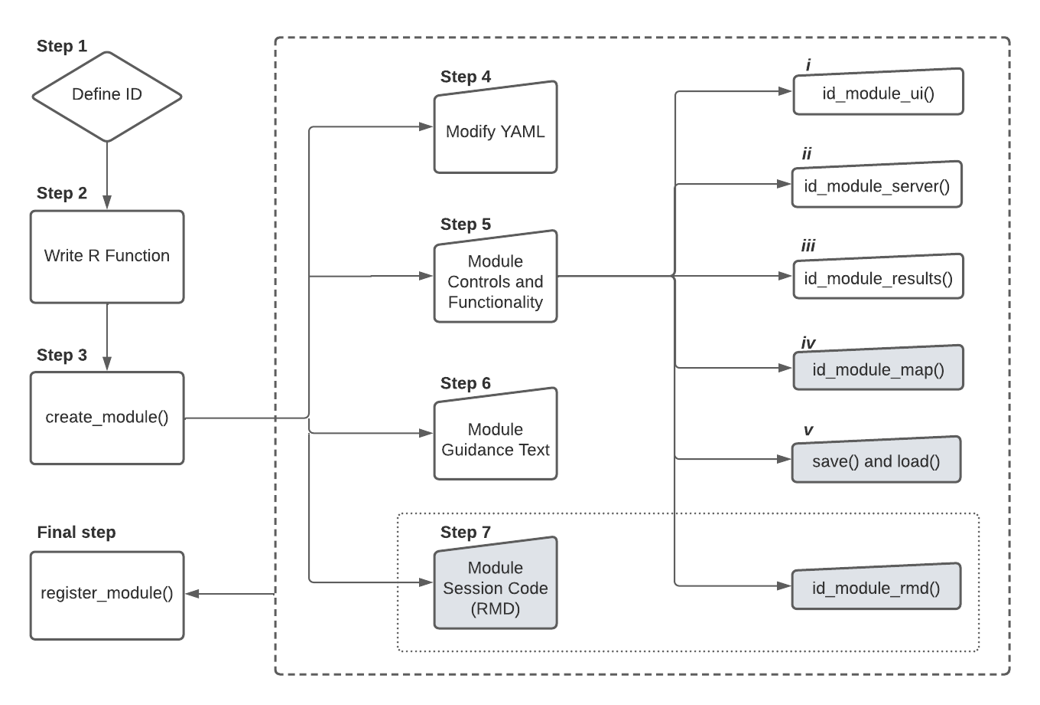
Module addition

There are seven necessary steps to adding a module:

Define an ID for the new module.
Write an R function.
Create a shiny module template using wallace::create_module(), which creates the four files .yml, .R, .md, and .RMD (the asterisk will be replaced by the module ID given when creating the template)
Modify the *.yml file to define internal parameters in Wallace. For example; the titles, authors, package used, and more importantly, the component in where your new module will be placed.
Add source code to the *.R file to display your module’s controls and implement its functionality.
Fill the *.Rmd with guidance text for your module.
Optional: Add session code to be incorporate in markdown to reproduce analysis in an R environment.
Tell the Wallace app to use your new module.

The example module we will describe calculates pairwise Pearson’s correlation coefficients for all environmental data, and will be added to the existing Process Environmental Data (penvs) component.

Step 1: Define ID

First, we must define an ID for the new module. This ID must be unique (there cannot be two modules with the same ID) and can only contain English letters, digits, and underscores.

New module IDs should begin with the short name for its component (e.g., “vis” for “Visualize”; see table below), followed by an underscore and a unique module short name.

Component	Short Name
Obtain Occurrence Data	occs
Obtain Environmental Data	envs
Process Occurrence Data	poccs
Process Environmental Data	penvs
Characterize Environmental Space	espace
Partition Occurrence Data	part
Build and Evaluate Niche Model	model
Visualize Model Results	vis
Transfer Model	xfer
Reproduce	rep

Examples of existing module names are occs_queryDb for the Obtain Occurrence Data component and the Query Database module, and poccs_thinOccs for the Process Occurrence Data component and the Spatial Thin module. The complete list can be found in the folder /wallace/inst/shiny/modules.

We will name this module “penvs_correlations”.

Step 2: Write an R function

Let’s write a function that carries out the module’s analysis. For this simple example, we will print a matrix of pairwise Pearson’s correlation coefficients for all environmental data. To calculate Pearson correlations among rasters, we will call the layerStats() function from the raster package (Hijmans & van Etten, 2012). This function takes the following inputs: 1) RasterStack of environmental data and 2) a statistic to compute (here we will use Pearson’s correlation coefficient). We will then write a module function to call the layerStats() function within the Wallace session.

This function has arguments for the 1) environmental rasterStack masked by the background extent (bgMask), 2) the name of the species (spN), and 3) logger, a reactive value object that holds all the text and HTML formatting for the log window. Reactive variables such as logger can only be used within reactive contexts – they will not work for regular R functions. When this function is run internally, the argument “logger” should be set to the reactive value object logger, which will get updated with the messages produced by our module function. This sends messages entered with writeLog() to the Wallace log window. The function smartProgress() will generate a shiny progress bar in the lower-right corner of the interface that tracks the progress of the layerStats() function. If the module function is run outside of a Wallace session, the argument “logger” should be left at the default NULL, which will make writeLog() and smartProgress() print messages and progress bars to the R console, respectively. Additionally, hlSpp() is a function that will highlight the printed text in bold green. This function should be used as the first parameter for writeLog() to highlight the printed species name (e.g., “Canis lupus | …Your message here…”).

Open a new R Script and write the module function as written below. This is a basic R function with some Wallace functionality that gets saved into the /R directory with the other package functions. Do not forget to document your function following basic roxygen structure with @export at the end, as we will need to include reference to this function in the NAMESPACE. Save the code below as wallace/R/penvs_correlations.R.

#' @title penvs_correlations
#' @description Runs Pearson correlations between variable pairs
#' @param bgMask Environmental rasters for study region.
#' @param spN Species' name for log window.
#' @param logger Reactive values list of log window text.
#’ @details Any additional details needed.
#' @return A data frame
#' @author Juan Perez

#' @export

penvs_correlations <- function (bgMask, spN = NULL, logger = NULL) {
  smartProgress(logger, 
                message = "Calculating pairwise Pearson's correlations", {
                  envCorrs <- layerStats(bgMask, 
                                         stat = "pearson", 
                                         na.rm = TRUE)
                })
  logger %>% writeLog(hlSpp(spN), "Pearson complete")
  return(envCorrs)
}

In the case that your function becomes too long or has many nested functions, you can write auxiliary (helper) functions in the same file (see wallace/R/envs_ecoClimate.R for an example).

Once your module function is finished, we will add it to the package NAMESPACE by running devtools::document() or by pressing Ctrl/Cmd + Shift + D in Rstudio. Finally, load the function using devtools::load_all().

Step 3: Create a shiny module with create_module()

We have just specified the functionality for the module, an .R script that goes in the /R folder, and now we will specify the module’s structure in several files that go in the /inst/shiny/custom_modules folder. Wallace modules depend on several files: *.yml, *.md, *.R, and optionally *.Rmd. To generate templates for these files, run wallace::create_module() , then fill the arguments in as follows:

id (string): It is the module name. You will use “penvs_correlations” here.
dir (string): Folder path in which your module will be saved. You will use “./inst/shiny/custom_modules”
result (boolean): TRUE for this example. TRUE if the module should support showing information in the Result tab. See more in Step 5, option iii.
map (boolean): FALSE for this example. TRUE if the module should support modifying the map. See more in Step 5, option iv.
save (boolean): FALSE for this example. TRUE if the module saves custom data when the user saves the current session. See more in Step 5, option v.
rmd (boolean): FALSE for this example. TRUE if the module should add Rmd code to the Session Code. See more in Step 7.

wallace::create_module(id = "penvs_correlations", 
dir = "./inst/shiny/custom_modules", 
map = FALSE,
result = TRUE, 
rmd = FALSE, 
save = FALSE)

Four new files will be created in the ./custom_modules directory: penvs_correlations.yml, penvs_correlations.md, penvs_correlations.R, and optionally penvs_correlations.Rmd.

Step 4: Modify YAML to internal module calling

Open the YAML file penvs_correlations.yml and set the following parameters:

component: Which component this module belongs to (one of: occs, envs, poccs, penvs, espace, part, model, vis, xfer)
short_name: The label to show beside the radio button in the component’s UI
long_name: A longer name for the module, to show as the title in the UI
authors: The author(s) of this module
package: The R package that is used by this module (if more than one, use a comma between them)

component: "penvs"
short_name: "Pearson's correlations"
long_name: "Calculate pairwise Pearson's correlations between environmental layers"
authors: "Peter Galante"
package: [raster]

Step 5: Module controls and functionality

Aside from the .R file in /R directory, you also need to have an .R file named penvs_correlations.R that specifies the controls and how the module function is run in the same directory as the YAML file. This R file contains 3 main parts and 3 optional ones:

A function named penvs_correlations_module_ui returns the user interface (UI) for this module, which includes the controls that the user interacts with to input module parameters and run functions. This function should follow the conventions for general Shiny modules—it should take a single argument called “id”, use it to create a unique namespace for the module, and return a list of UI objects. Usually, there should at least be a button that runs the module function. Shiny modules operate in their own unique namespaces, and so use of the NS() function is necessary to ensure the module’s UI controls can talk to ui.R. The function ns() (for namespace), returned from NS(id), is run on the ID names of shiny UI input elements, as in numericInput(ns("degFr"), ...), to enable this connection to ui.R. See the shiny module vignette for more details.

penvs_correlations_module_ui <- function(id) {
  ns <- shiny::NS(id)
  tagList(
    # UI
    ## Add a checkbox for batch processing (more than 1 species)
    checkboxInput(ns("batch"), label = strong("Batch"), value = TRUE),
    ## Give the action button a name and a label.
    actionButton(ns("runCorrs"), label = "Calculate correlations"),
    ## UI for reselecting variables after calculating correlations. This custom input one will create in the server module function
    uiOutput(ns("VarSelect")),
    ## UI button to select variables to be used in the analysis.
    actionButton(ns("selectConfirm"), label = "Select Variables")
    )
}

A function named penvs_correlations_module_server that defines the server functionality for this module. This function should follow the conventions for general Shiny modules— it should take arguments input, output, and session, as well as one extra argument common.

The common variable supplied to a module’s server function (and map function, explained later) is a list containing: The following reactive variables that can be used by the module: logger, spp, curSp, allSp, curEnv, curModel, component, module, envs.global, mapCntr. The following reactives that are shortcuts to reactives inside spp: occs, envs, bg, bgExt, bgMask, evalOut, mapPred, mapXfer, rmm. A function update_component(tab) that allows you to switch to a new tab within the component.

This function penvs_correlations_module_server() is a wrapper for a shiny reactive expression. Inside, there is a template for the essential parts needed in a Wallace module. First, we specify shorter names for the shortcut variables inside the “common” list. Next, we specify a UI function that can use reactive values inside of this server function—in this case, we want to know the names of the environmental variables input so they can be printed to the UI control (see Creating a reactive shortcut in the next section for more details). After this, we specify when the module function gets run. The function observeEvent() performs an action in response to an event (e.g., clicking a button created by penvs_correlations_module_ui()). Inside of each observeEvent(), you need to include the following code. The first, “WARNING”, catches any possible errors before the module’s core functionality is run. If there is an error, the function stops and a log error message is written. The user will need to define these errors in order to catch them and prevent the module from crashing unexpectedly. Next, under “FUNCTION CALL”, we call the function from /wallace/R and make sure it returns what we expect. Next, under “LOAD INTO SPP”, we load the model object into spp. Finally, under “METADATA”, we fill in appropriate metadata fields for the rangeModelMetadata object in spp. Ultimately, the module author decides what metadata to include, but we encourage authors to explore the rangeModelMetadata object, decide which fields best apply to your module, and enter information detailed enough to enable reproducibility. As shiny modules exist in their own namespaces, if we want to refer to any of the results from the module later (in other modules), we need to put them into the spp reactiveValues list.

penvs_correlations_module_server <- function(input, output, session, common) {
  ## Define common objects that will be used in this function
  logger <- common$logger
  spp    <- common$spp
  allSp  <- common$allSp
  curSp  <- common$curSp
  bgMask <- common$bgMask # raster stack after masking by background
  VarSelector <- common$VarSelector # See how to create and include a reactive shortcut later in the main text.

  # Create a custom UI input
  output$VarSelect <- renderUI({
    req(bgMask())
    shinyWidgets::pickerInput(
      "VarSelector",
      label = "Select variables",
      choices = setNames(as.list(names(bgMask())), names(bgMask())),
      multiple = TRUE,
      selected = names(bgMask()),
      options = list(`actions-box` = TRUE))
  })

## When action button defined in the ui function above is clicked, do the following:
  observeEvent(input$runCorrs, {
     # WARNING ####
    if (is.null(bgMask())) {
      logger %>% writeLog(type = 'error', hlSpp(curSp()), 'Background data missing. Sample study region first')
      return()
    }
    # Check that the background has already been selected
    req(bgMask())
       
    # Set up if you want batch to be allowed
      # allSp() is the list of species selected
      # curSp() refers to the currently selected species in the GUI
    if (input$batch == TRUE) spLoop <- allSp() else spLoop <- curSp()
    # If batch is true, loop through all species (allSp())
    for (sp in spLoop){
    # FUNCTION CALL ####
      smartProgress(logger, message = "Calculating pairwise correlations", {
        envCorrs <- raster::layerStats(x = spp[[sp]]$procEnvs$bgMask, na.rm = T, stat = "pearson")})
    # To update the log window
    logger %>% writeLog(hlSpp(sp), "Finished calculating correlations")
    #envCorrs <- raster::layerStats(x = bgMask(), na.rm = T, stat = "pearson")

    # LOAD INTO SPP ####
  spp[[sp]]$procEnvs$envCorrs <- envCorrs$`pearson correlation coefficient`

    # METADATA ####

  }
  # Switch to Results tab to display results
  common$update_component(tab = "Results")
  })

  # Define output as a table
  output$envCorrTable <- renderText({
    # Result
    knitr::kable(spp[[curSp()]]$procEnvs$envCorrs, format = 'html')
  })

  ## Observe when selection is confirmed
  observeEvent(input$selectConfirm, {
    req(spp[[curSp()]]$procEnvs$envCorrs)

    ## update bg object
    spp[[curSp()]]$procEnvs$bgMask <- spp[[curSp()]]$procEnvs$bgMask[[VarSelector()]]

    # Add a line to logger to identify which variables were selected
        # hlSpp() prints the species name in green, bold, and italics
    logger %>% writeLog(hlSpp(curSp()), "Selected: ", paste0(names(spp[[curSp()]]$procEnvs$bgMask), collapse = ", "))
  })
}

Creating a reactive shortcut

The custom UI slot (“varSelector”) in the server function (penvs_correlations_module_server) requires the names of the selected variables that were uploaded in the previous component (e.g., WorldClim, ecoClimate, user-specified). Because the numbers and names of the rasters will change depending on which rasters were uploaded, we need to create a reactive function to get their names. In addition to writing the code to make this UI object in the server file above, we additionally need to add two lines to the main “inst/shiny/server.R” file.

The first line creates the reactive object. For organizational purposes, reactive shortcuts should be placed with the other shortcuts created in each component. Please add only the last line in the “COMPONENT: PROCESS ENVIRONMENTAL DATA” section, which should be at line #380.

  ############################################## #
  ### COMPONENT: PROCESS ENVIRONMENTAL DATA ####
  ############################################## #

  # # # # # # # # # # # # # # # # # #
  # PROCESS ENVS: other controls ####
  # # # # # # # # # # # # # # # # # #

  # convenience function for background points table for current species
  bg <- reactive(spp[[curSp()]]$bg)
  # convenience function for background polygon for current species
  bgExt <- reactive(spp[[curSp()]]$procEnvs$bgExt)
  # convenience function for environmental variable rasters masked to background for current species
  bgMask <- reactive(spp[[curSp()]]$procEnvs$bgMask)
  # THIS LINE WILL CREATE THE REACTIVE
  VarSelector <- reactive(input$VarSelector)

The second line will add the shortcut to the common list. Please search for “COMMON LIST FUNCTIONALITY” (#1310) in the server file, and add it to the section of “Shortcuts to values nested inside spp”.

  ################################
  ### COMMON LIST FUNCTIONALITY ####
  ################################

  # Create a data structure that holds variables and functions used by modules
  common = list(
    # Reactive variables to pass on to modules
    logger = logger,
    spp = spp,
    curSp = curSp,
    allSp = allSp,
    multSp = multSp,
    curEnv = curEnv,
    curModel = curModel,
    component = component,
    module = module,
    envs.global = envs.global,
    mapCntr = mapCntr,

    # Shortcuts to values nested inside spp
    occs = occs,
    envs = envs,
    bcSel = bcSel,
    ecoClimSel = ecoClimSel,
    bg = bg,
    bgExt = bgExt,
    bgMask = bgMask,
    bgShpXY = bgShpXY,
    selCatEnvs = selCatEnvs,
    evalOut = evalOut,
    mapPred = mapPred,
    mapXfer = mapXfer,
    rmm = rmm,
    VarSelector = VarSelector, # ADD line here (do not forget to add a comma at the end)

A function named penvs_correlations_module_result that returns the UI output for the results of the module function (i.e., plot, table). Any outputs need to be rendered in the penvs_correlation_module_server function, and the ID name of these outputs are specified here (in this scenario, output$envCorrTable). This function should also follow the same conventions regarding module namespace as the previous functions.

penvs_correlations_module_result <- function(id) {
  ns <- NS(id)
  # Result UI as html
  htmlOutput(ns("envCorrTable"))
}

OPTIONAL: A function named penvs_correlations_module_map that modifies the map. This function takes two arguments: map (a reference to a leaflet map) and common (the same parameter from the server function).
OPTIONAL: The penvs_correlations_module_server function can enable the module to record the session information when the session is saved. This option will be enabled when you specified the parameter save as TRUE when using create_module(). It returns a list with two functions: save() and load(state). The save() function takes no arguments and should return a named list with all the variables to save. The load(state) function takes one argument, which should consist of the same list of variables that were saved.

Step 6: Guidance text for your module

The last vital step is writing guidance text for your module. This text provides a detailed description of what your module does and where to find more relevant information for the benefit of other users. To add these instructions and other information for your module, you need to edit the Markdown file penvs_correlations.md. Enter the background information for the module’s analysis, any methodological details that help users understand what the module does and why they might want to use it, and any relevant references to the literature. Guidance texts have three sections. BACKGROUND provides general information about the framing of the module’s technique in the grand scheme of things. IMPLEMENTATION describes how the technique is used in this module. Finally, REFERENCES is a bibliography of academic sources that are referenced in the text.

### **Module: Pearson Correlation**

**BACKGROUND**

Calculate pairwise Pearson's product-moment variable correlations for all predictor variables. 

**IMPLEMENTATION**

After loading environmental layers select background extent and sample background points. These points are used to sample each layer to calculate correlations. Correlations are calculated for single or multiple species.

**REFERENCES**

Robert J. Hijmans (2019). raster: Geographic Data Analysis and Modeling. R package version 2.9-5.

Step 7: Session code to reproduce analysis in an R environment

OPTIONAL: A function named penvs_correlations_module_rmd that adds code to the “Session Code” Rmd output to enable reproducibility of your module analysis. This function returns a list with variables that are used in the module’s RMD code, and takes an argument species that contains all the information for the current species. If you specified the rmd parameter as TRUE in create_module() from Step 3, the file template penvs_correlations.Rmd will be created in the custom_module directory. You should add code to this RMD file to repeat the module analysis. If you need to use any variables originally specified by the user during the session, you can use double curly brackets and define it inside the penvs_correlations_module_rmd function. For example, in modules/occs_queryDb.R line #169, the number of occurrences to download from gbif (occs_queryDb module) is saved in occNum_rmd. Then, see line #16 in modules/occs_queryDb.Rmd to find the same object with curly brackets, {{occNum_rmd}}, is used to create the specific session code of the module. Two variables are always made automatically available for these RMD code chunks: {{sp}} is the species ID and {{spName}} is the species’ scientific name. See other module RMD files for examples in inst/shiny/modules.

Final step: Tell the Wallace app to use your module

Congratulations! You finished creating your module. The final step is to tell the Wallace application to use it by calling the register_module() function.

wallace::register_module("./inst/shiny/custom_modules/penvs_correlations.yml")

Then, you just need to open Wallace using run_wallace() and your new module is ready for a test drive!

Gonzalo Pinilla-Buitrago, Jamie M. Kass, Siew Fong Chen, Peter Galante, Bethany A. Johnson, Dean Attali

April 19, 2022