Wallace Ecological Modeling Application v2.0 Vignette

This work is distributed under the CC-BY-NC-SA 4.0 license.

Preface

Welcome to the Wallace EcoMod v2.0 vignette. This vignette was written specifically for v2.0, so if you are using a different version, some things may not match up. Click here for the v1.0 vignette or here for this vignette in Spanish.
Additionally, we anticipate that this vignette (and those in the future) for the wallace package will be updated or appended regularly in accordance with ongoing development.

Introduction

Wallace is an R-based GUI application (R package wallace) for ecological modeling that currently focuses on building, evaluating, and visualizing models of species niches and distributions. We will refer to these models as species distribution models (SDMs), and we will not explain them at length here—as you read through, you will be pointed to some sources of detailed information within the application (such as the Component Guidance and Module Guidance tabs) for reference.

Wallace has many qualities which we think make it a good example of next-generation scientific software: it’s 1) accessible, 2) open, 3) expandable, 4) flexible, 5) interactive, 6) instructive, and 7) reproducible.

The application, which is constructed with the R package shiny, features a pannable/zoomable map and dynamic plots and tables. Data for the models can be downloaded from online databases or uploaded by the user. Most results can be downloaded, including the option to save R code that can reproduce your analysis. For more details, including on SDMs, please see our initial publication¹ in Methods in Ecology and Evolution and our follow-up publication² in Ecography.

Kass, J.M., Vilela, B., Aiello-Lammens, M.E., Muscarella, R., Merow, C., Anderson, R.P. (2018). Wallace: A flexible platform for reproducible modeling of species niches and distributions built for community expansion. Methods in Ecology and Evolution, 9(4),1151-1156. https://doi.org/10.1111/2041-210X.12945
Kass, J.M., Pinilla-Buitrago, G.E, Paz, A., Johnson, B.A., Grisales-Betancur, V., Meenan, S.I., Attali, D., Broennimann, O., Galante, P.J., Maitner, B.S., Owens, H.L., Varela, S., Aiello-Lammens, M.E., Merow, C., Blair, M.E., Anderson R.P. (2022). wallace 2: a shiny app for modeling species niches and distributions redesigned to facilitate expansion via module contributions. Ecography, 2023(3), e06547. https://doi.org/10.1111/ecog.06547.

The Wallace project’s main page has links to the Google Group, the official email, the CRAN page hosting the stable version, and the GitHub development page. Wallace also has a YouTube channel with various tutorial videos and recorded seminars.

If you use Wallace in your teaching, we would like to hear about your experiences. Please take a moment to complete the short survey: Wallace external workshop and curriculum survey.

Setup

Installing the package

For wallace to work, you should be using R version 3.5.0 or later. Download for Windows or Mac.

To install and load Wallace v2.0.6, open either the R GUI or RStudio and run the code below. It’s the only code you’ll have to run to use wallace.

# Install Wallace from CRAN
install.packages("wallace")

# OR install Wallace from GitHub
install.packages("remotes")
remotes::install_github("wallaceEcoMod/wallace")

# THEN load Wallace
library(wallace)
# AND Run Wallace
run_wallace()

The Wallace GUI will open in your default web browser, and the R console will be occupied while Wallace is running.

The R console displays messages regarding R-package information or any error messages if complications arise, including valuable information for troubleshooting. If you intend to ask a question in the Google Group (preferred) or by email, please include any errors messages from the console.

If you’d like to use the R console while running Wallace, open another R session, or alternatively a terminal window (MacOS/Linux) or command prompt (Windows) and initialize R, then run the lines above.

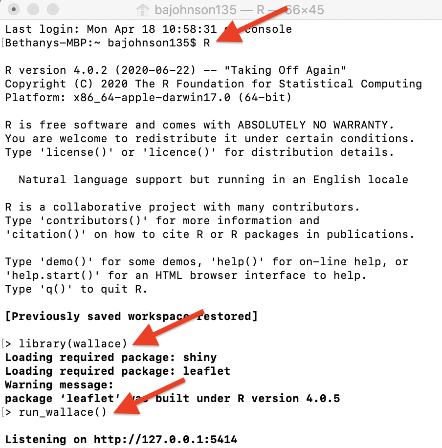
An example with Terminal in MacOS.

To exit Wallace, hit ‘Escape’ while in the R console and close the browser window, or click the quit button in the top right corner of the GUI. Note: If you close the browser window running Wallace, your session will be over and all progress will be lost. See Save & Load Session for how to save your work and be able to restart your analysis.

Setting up Java version of Maxent

Wallace v2.0 includes two options to run Maxent models: maxnet and maxent.jar. The former, which is an R implementation of Maxent and fits the model leveraging the package glmnet, is now the default and does not require running Java (see Phillips et al. 2017). The latter, which is the original Java implementation, runs the maxent() function in the package dismo, which in turn relies on tools from the package rJava. When using dismo to run maxent.jar, the user must place the maxent.jar file in the /java directory of the dismo package root folder. You can download Maxent here and find maxent.jar, which runs Maxent, in the downloaded folder. You can find the directory path to dismo/java by running system.file(‘java’, package=“dismo”) in the R console. Simply copy maxent.jar and paste it into this folder. If you try to run Maxent in Wallace without the file in place, you will get a warning message in the log window and Maxent will not run. Also, if you have trouble installing rJava and making it work, there is a bit of troubleshooting on the Wallace Github repository README that hopefully should help.

Orientation

We’ll begin with an orientation of the Wallace interface. After running run_wallace(), Wallace opens to the Intro page. The “About” tab contains background information about the program. The “Team” tab has details about the developers and collaborators who contributed to Wallace. The “How to Use” tab contains a brief user manual, which is an abridged version of this vignette without a worked example. The “Load Prior Session” tab is for loading a prior session, which we will cover later.

At the top in the orange panel are the Components, which represent the steps of analysis. Each of these component tabs opens to the corresponding step. Within each component are several Modules, which are discrete analysis options within the components. To the left in the gray panel is the Wallace WORKFLOW, outlining the version number, components (numbered), and modules (bulleted) currently included.

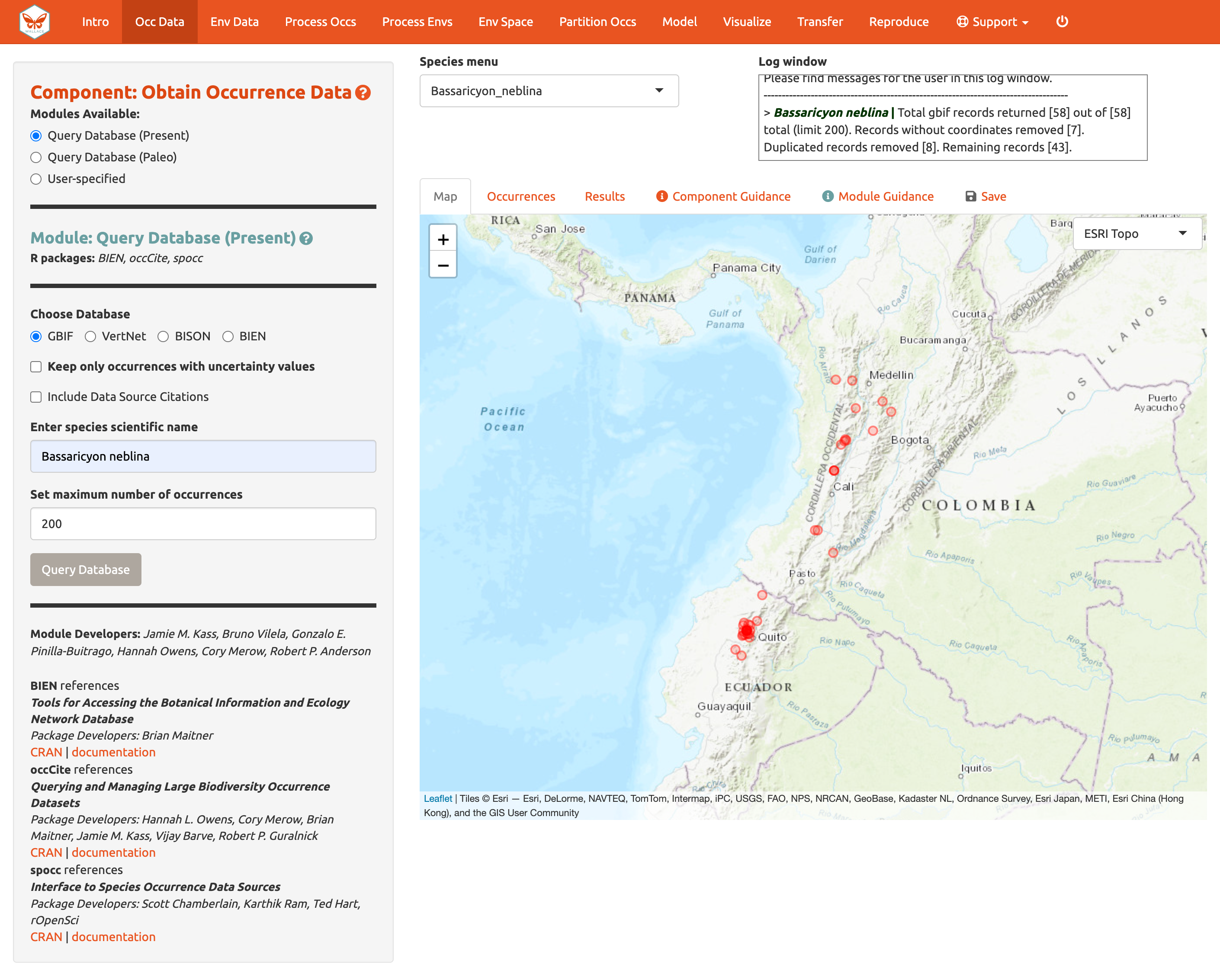
Click on the component tab Occ Data, select a module, and consult the schematic below showing the different parts of the Wallace interface.

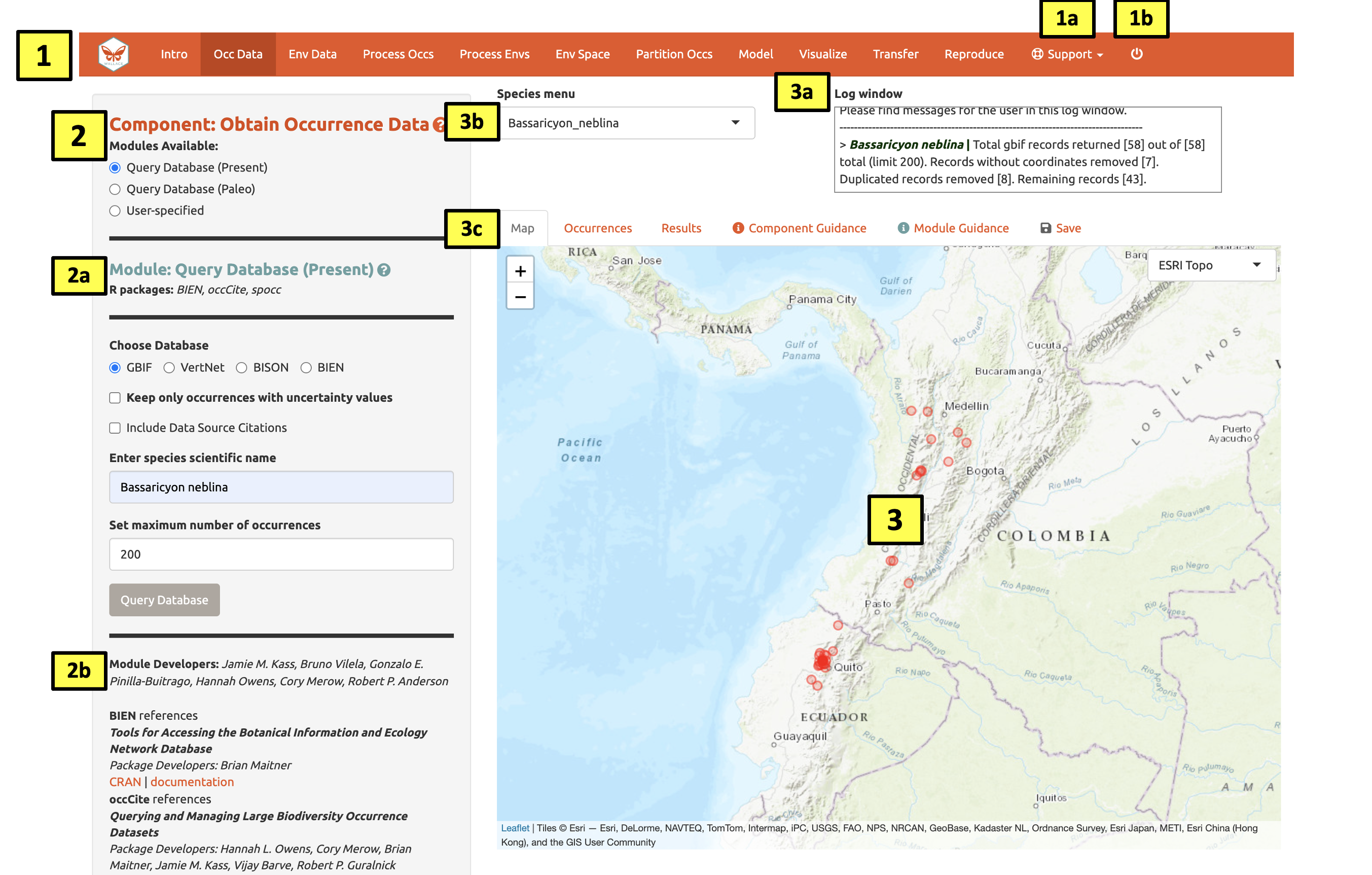
(1) These are the components. You will be stepping sequentially through them. Wallace v2 now includes a Support button (1a), which links to the Google Group, email, website, and the Github page to report issues, as well as the quit button (1b), which will end the session.
(2) This is the toolbar with all the user interface controls, such as buttons, text inputs, etc. You can see that the module Query Database (Present) is currently selected. You’ll see that two other modules exist for this component: Query Database (Paleo) and User-specified. This last module lets you upload your own occurrence data. Try choosing it instead and notice that the toolbar changes, then click back to Query Database (Present).
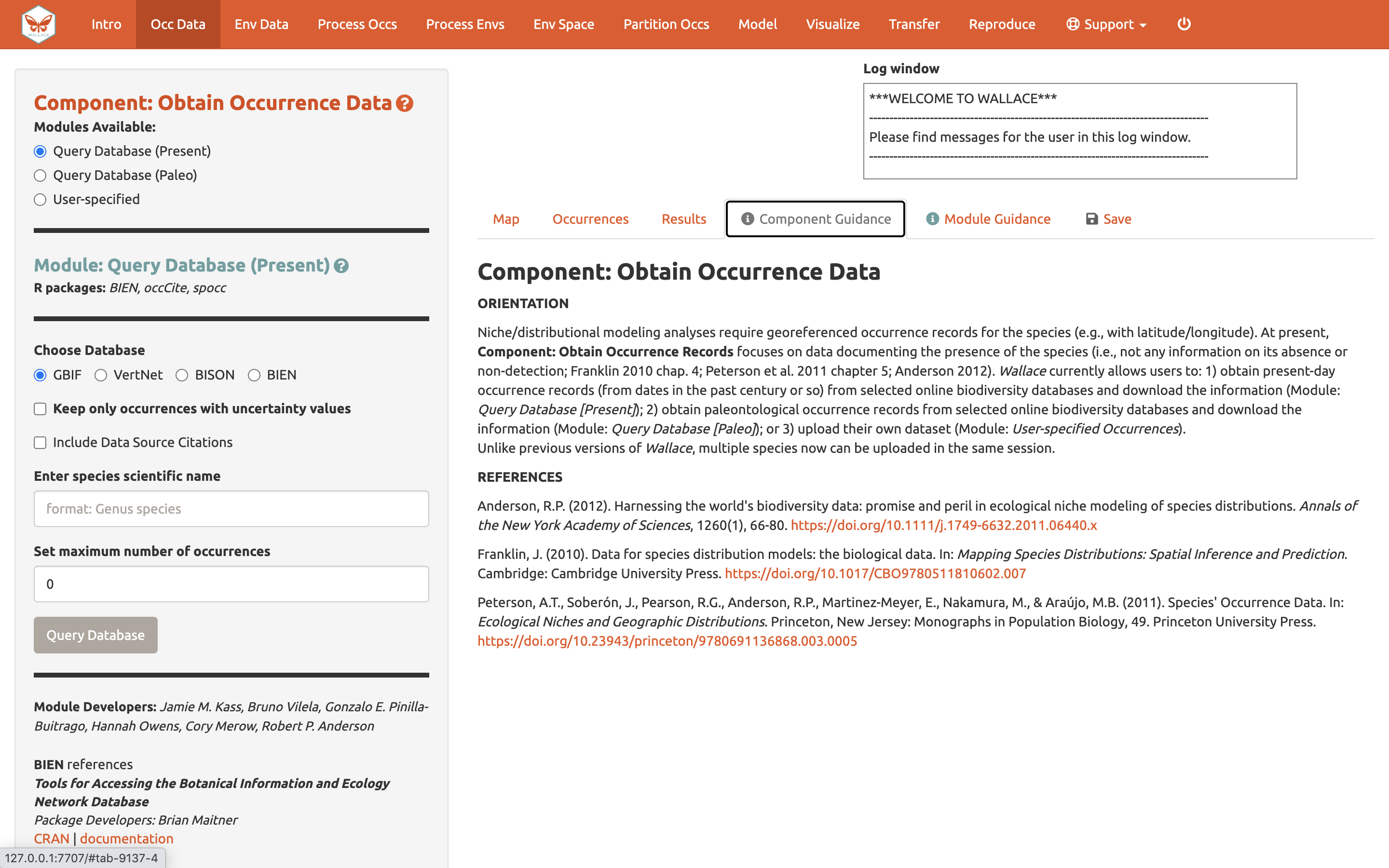
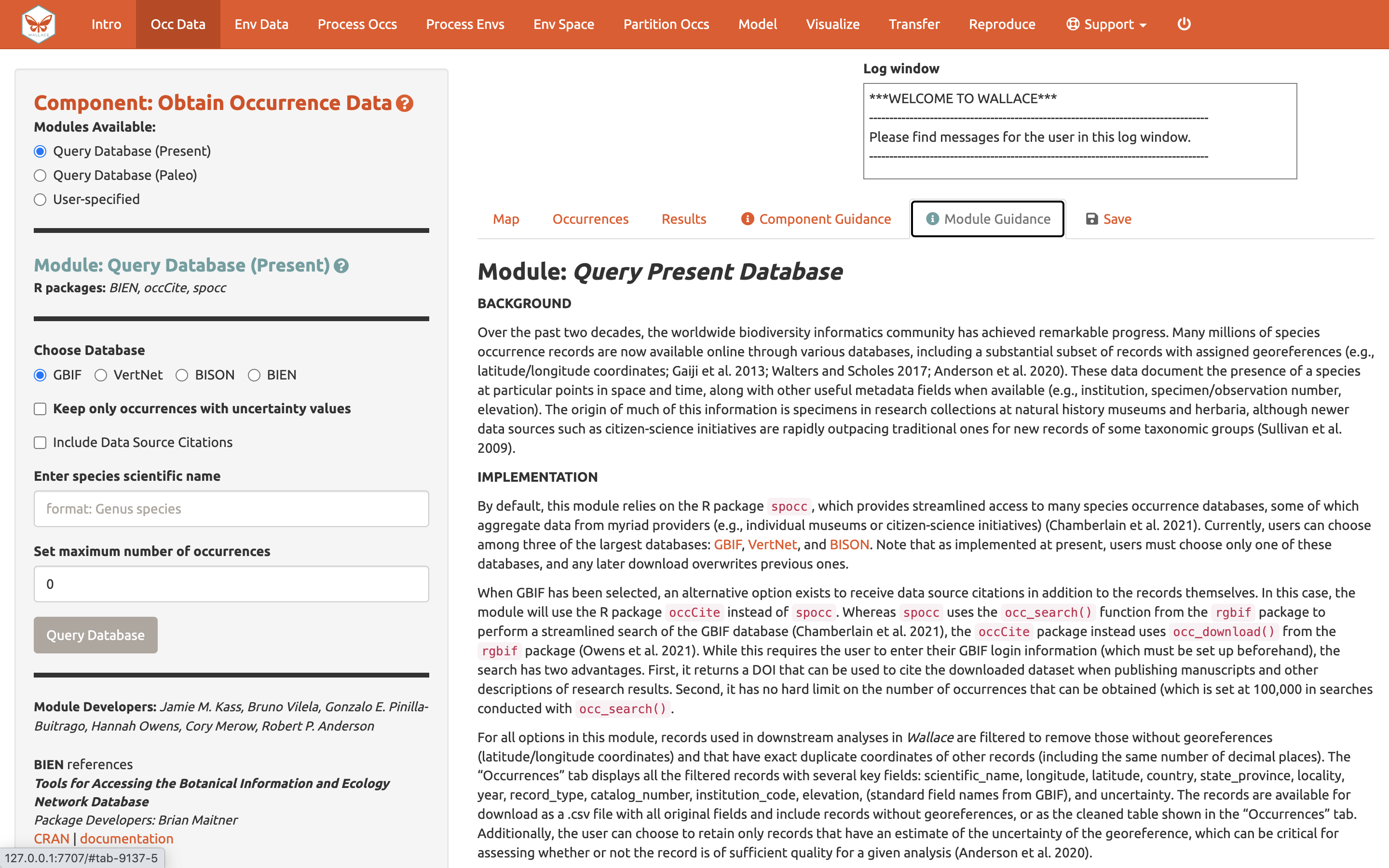
Both the Component and Module have question mark buttons (?) next to the title text. Clicking these will link to the respective guidance texts.
Within this toolbar, you can find the module name and the R packages it uses (2a), as well as the control panel for the selected module (2b). Modules can be contributed by other researchers and the developers; CRAN links and documentation are at the bottom.
(3) The right side is the visualization space. Any functions performed will trigger a message in the log window (3a). This window will also display any error messages. Wallace v2.0 now allows the user to load multiple species. If multiple species are loaded, toggle and select between species using the species drop-down menu (3b).
The visualization space includes several tabs (3c), including an interactive map, occurrence records table, results window, model and component guidance text windows, and a tab for saving outputs and the current session.

At this stage of the analysis, no results exist, and you have no data yet for the table, but you can view the Component Guidance and Module Guidance text now. This text was written by the developers to prepare users for each component and module theoretically (why we should use the tools) and methodologically (what the tools do). The guidance text also references scientific papers from the literature for more detailed reading. Please get into the habit of consulting these before undertaking analyses—and discussing them with your peers—-as this should give you a more solid foundation for moving forward.

The next tab in the visualization space is Save. At any point along the workflow, selecting “Save session” within this tab will save the progress as a .rds file. This file can be loaded back into wallace to resume analysis. If at any point during the vignette you need to pause, jump to Save & Load Session to learn how to save and load your Wallace session. This tab is also where you will be able to download and save results. The session code, metadata, and package citations can be downloaded within Component: Reproduce.

Now let’s begin our analysis.

We’ll be modeling the ranges of two mammal species of the genus Bassaricyon, which are members of the family Procyonidae that includes raccoons. Bassaricyon neblina, or the olinguito, is found in tropical montane areas of western Colombia and Ecuador in South America. The olinguito gained species status in 2013 when it was identified from existing museum specimens and is currently a species of concern listed as “Near Threatened” by the IUCN (Helgen et al. 2020). Bassaricyon alleni, or the eastern lowland olingo, is a relative of the olinguito and has a broader range throughout northern South America; it is currently listed as “Least Concern” by the IUCN (Helgen et al. 2016).

Obtain Occurrence Data

Make sure you are in the first component (Obtain Occurrence Data) and click to read the component guidance text. There are three modules available for obtaining occurrence data: Query Database (Present), Query Database (Paleo), and User-Specified. Choose a module and click on the module guidance text. Notice the module guidance text changes as you select among the three modules. Read through these to get a better understanding of how occurrence data is typically obtained and how wallace implements it.

Note: As of 01 September 2023, Module: Query Database [Paleo] will be temporarily unavailable.

Let’s proceed to get some occurrence data. We’ll be using present occurrences (as opposed to those from the deep past via fossil data, etc.) and therefore use Module: Query Database (Present). There is a selection of databases to choose from, as well as the option to return only those occurrences that contain information on coordinate uncertainty (which can be useful to filter by later). If you have a GBIF User ID, checking the “Include Data Source” box will allow you to log in with your username and password to download a DOI for the dataset. In order for this to work, you will need to install the R-package occCite prior to running Wallace. Since occCite is a suggested package, it will not install automatically like the other package dependencies.

Choose GBIF (the Global Biodiversity Information Facility—one of the largest storehouses for biodiversity data), keep uncertainty unchecked, type in Bassaricyon neblina into the scientific name box, set the maximum number of occurrences to 200, and click Query Database.

After the download is complete, the log window will contain information on the analysis performed. Your search should return at least 58 records (numbers recorded at the time of writing), but after accounting for records without coordinate information (latitude, longitude) and removing duplicate records, at least 43 should remain. This species has relatively few records, so setting the maximum to 200 is sufficient, but for modeling with data-rich species, 200 may not be enough for adequately sampling the known range, and the maximum can be increased. **Numbers may be different as more records are added to GBIF.

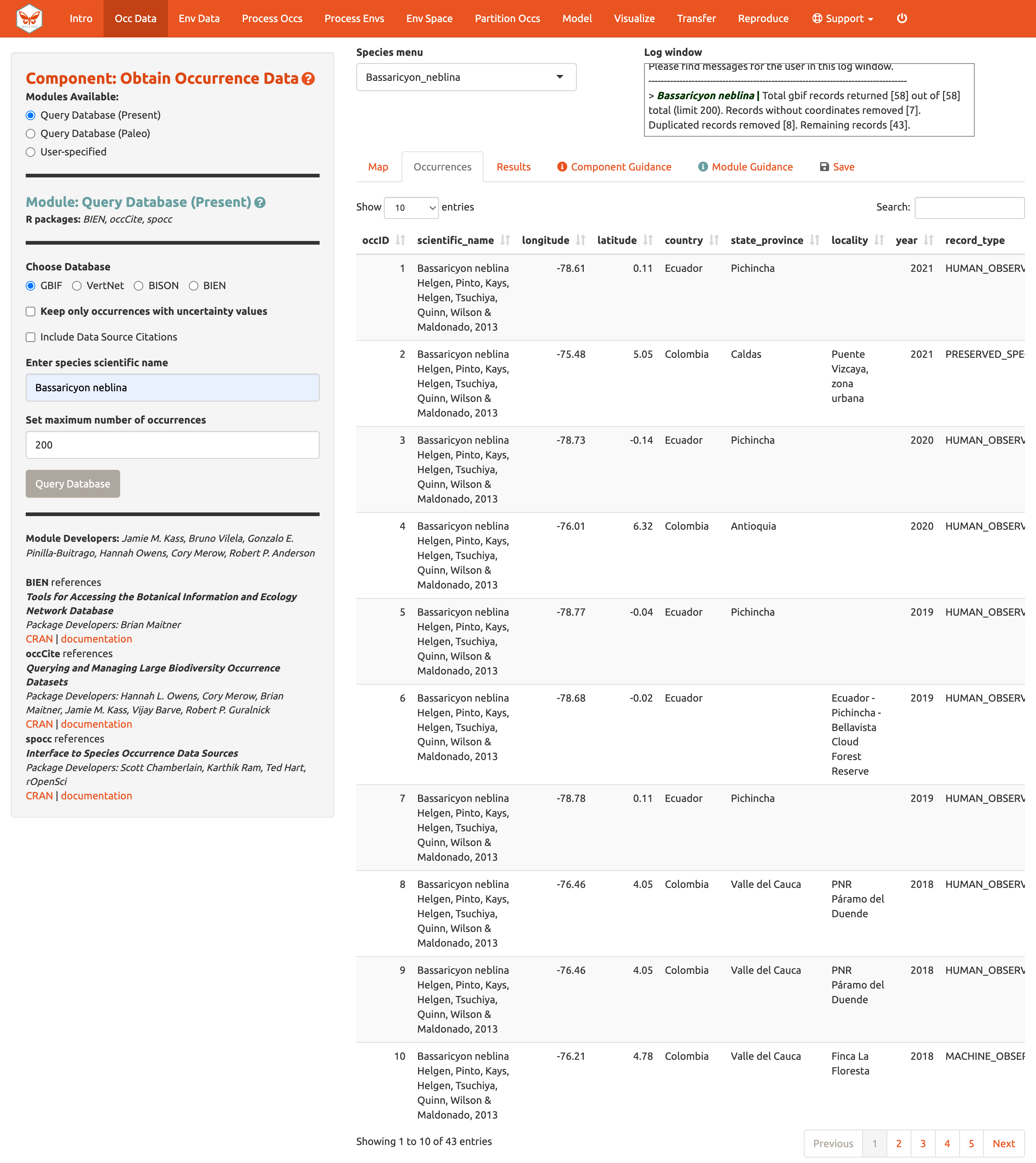
Now click on the “Occurrences” tab to view more information on the records. The developers chose the fields that are displayed based on their general relevance to studies on species ranges. Note that you can download the full table with all fields.

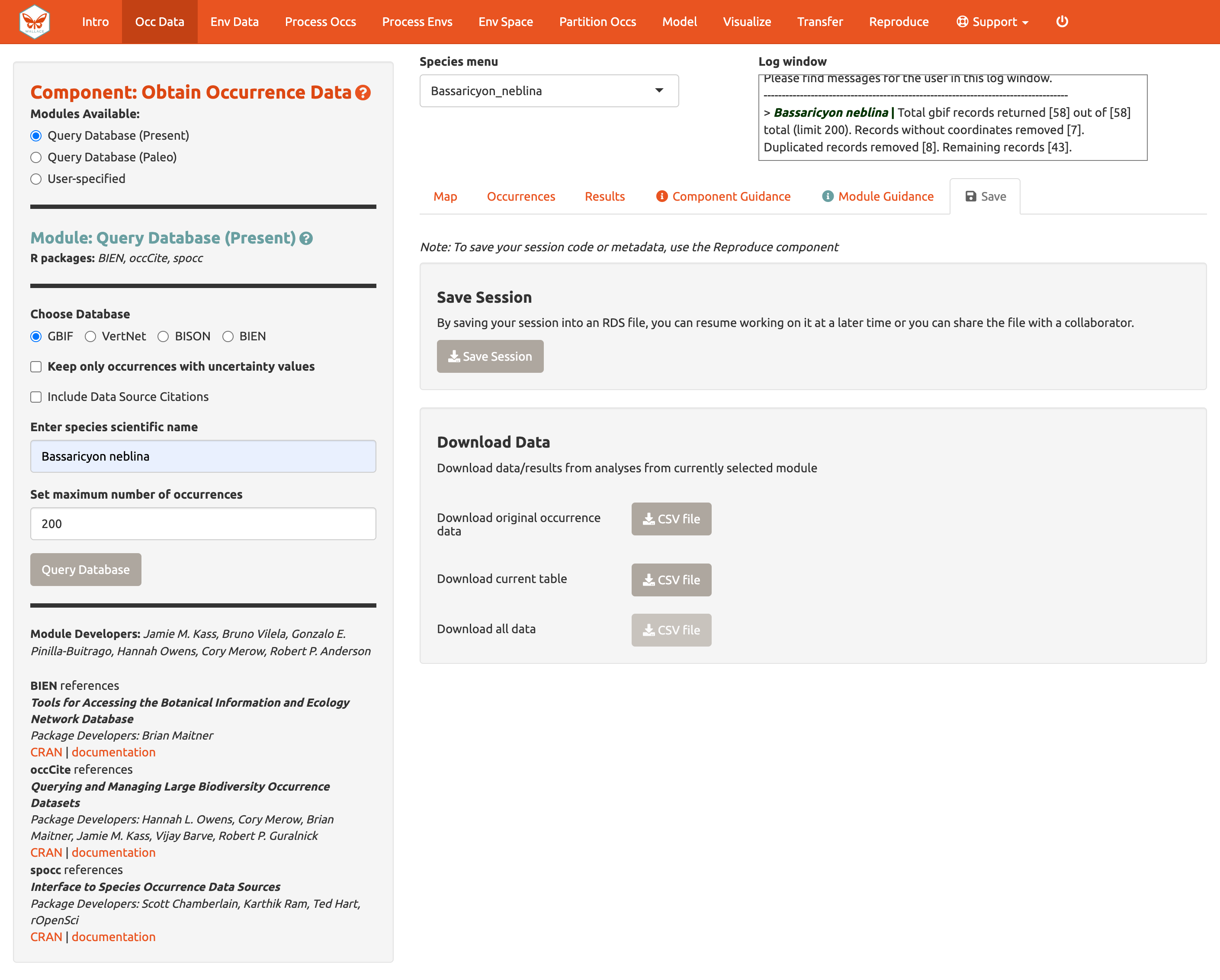
Click the “Save” tab. The first save box allows you to download your session. It is available in all the components and modules (See Save & Load Session section for more details). The download options below the Save Session box change depending on which component is selected. Here, you can get a .csv file of the records just acquired. The first option will download the original database fields for every downloaded record (before any filtering). The second option downloads the current table. The third option, “Download all data”, is unavailable at this point, but that will change after we include our second species.

Note to Chrome users: If you find the map is loading incorrectly after downloading an object, specifically the corner tile loads but the rest of the map is gray, closing the download bar at the bottom of the page should reset the map and fix the problem.

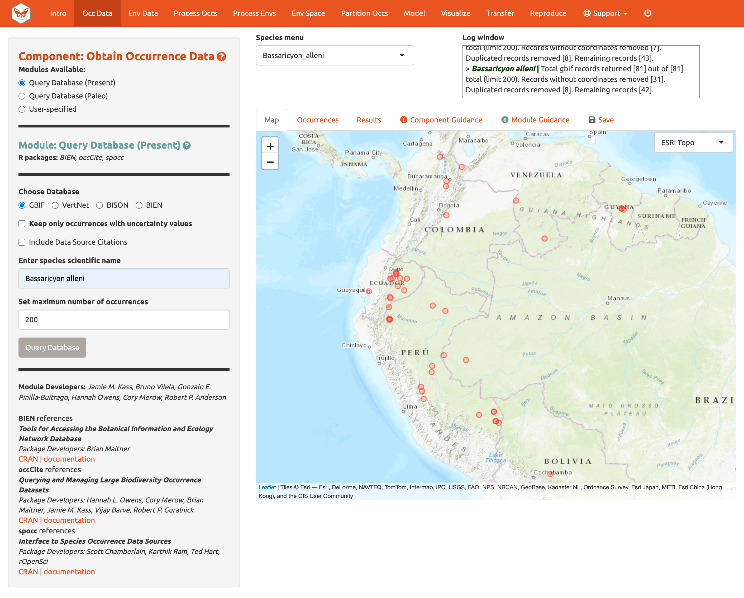
A major improvement in Wallace v2.0 from previous versions is the ability to consider multiple species (separately) in the same session. Let’s add another species to model.

Aside from GBIF, you can query the Vertnet (for vertebrate data) and newly added BIEN (for botantical data) for species occurrence records. In the second module Query Database (Paleo), you can query PaleobioDB databases for fossil records by selecting a time interval and species. Specific packages may have to be downloaded prior to loading Wallace to use these (e.g., BIEN and paleobioDB).

If you have your own occurrence data, you can import it using the third module, User-specified. Your occurrence data file must be a .csv with the columns “scientific_name”, “longitude”, and “latitude”, explicitly named and in that order. It may have other columns, but those must be the first three. You also have the option to specify the delimiter and separator of your file.

We’ll continue with GBIF occurrence data. Search the database for Bassaricyon alleni (eastern lowland olingo), keeping the max set at 200. This should return at least 81 records and after cleaning should come to at least 42 records. You might have noticed that the log window was updated, but the map remains the same. The map will not change automatically, as Bassaricyon neblina is still selected in the Species menu. Toggle between species to show the map for Bassarricyon alleni.

Click back to the “Save” tab. Notice that the third option is now available.

Obtain Environmental Data

Next, you will need to obtain environmental variables for the analysis. The values of the variables are extracted for the occurrence records, and this information is provided to the model. These data are in raster form, which simply means a large grid where each grid cell specifies a value. Rasters can be displayed as colored grids on maps (we’ll see this later). Click on the component Env Data. The first module, WorldClim Bioclims, lets you download bioclimatic variables from WorldClim, a global climate database of interpolated climate surfaces derived from weather station data at multiple resolutions. The interpolation is better for areas with more weather stations (especially in developed countries), and more uncertainty exists in areas with fewer stations. The bioclim variables are summaries of temperature and precipitation that have been proposed to have general biological significance. You have the option to specify a subset of the 19 total variables to use in the analysis.

The second module, ecoClimate, is a module included with v2 that includes paleoclimate reconstructions. It accesses climatic layers from the PMIP3 – CMIP5 projects from ecoClimate. Users can select from Atmospheric Oceanic General Circulation Models and choose a temporal scenario to use. All ecoClimate layers have a resolution of 0.5 degrees, whereas WorldClim allows resolution options of 30 arcsec, 2.5 arcmin, 5 arcmin, or 10 arcmin.

The third module, User-specified, is for uploading your own rasters into Wallace. These can be continuous, numerical, or categorical variables to provide to the model.

We’ll be using WorldClim. The first time you use Wallace, these data are downloaded to a temporary folder on your hard drive; after that, they will simply be loaded from this local directory (which will be quicker than downloading from the web). You also have the option to save to memory for faster processing–this saves the data temporarily as a RasterBrick in your RAM for Wallace to access. Finer resolution rasters will take longer to download. 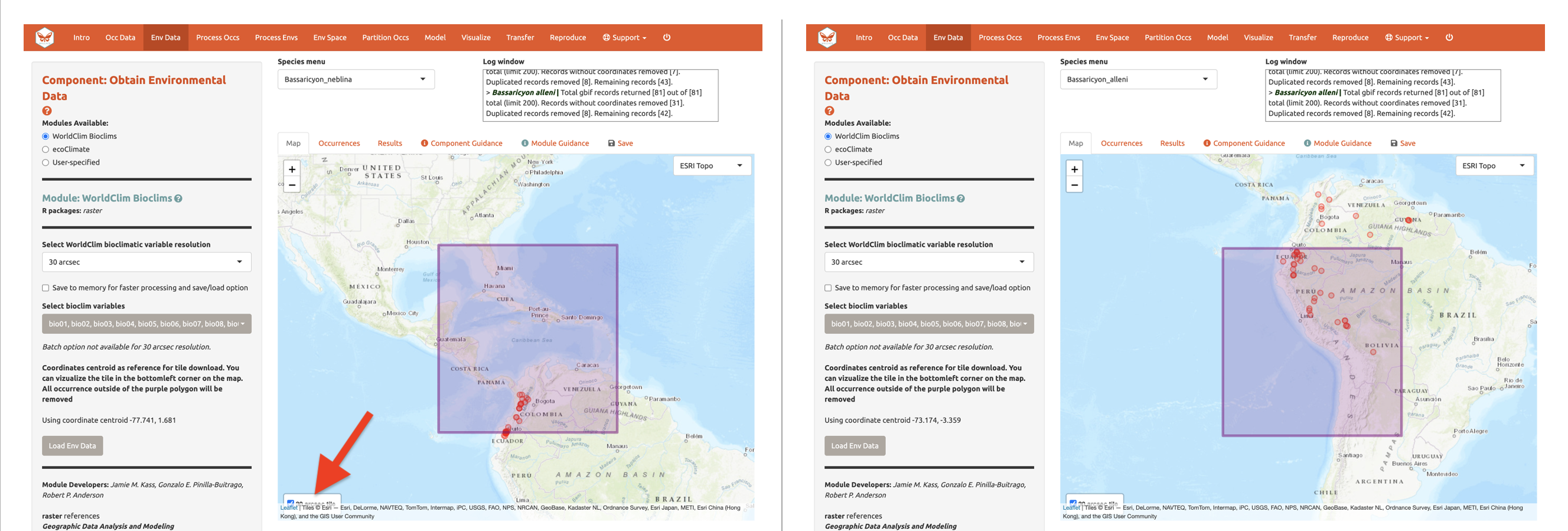The finest resolution data (30 arcsec) is served in large global tiles when downloading through R with the raster package (which wallace uses) and a single tile that corresponds to the map center will be downloaded. Set the resolution to 30 arcsec and the latitude and longitude of the map center will be given. To visualize how well the tile will cover the occurrence points, click the “30 arcsec tile” box in the bottom left corner of the map. The points outside the tile will be excluded; you may need to zoom out to see fully.

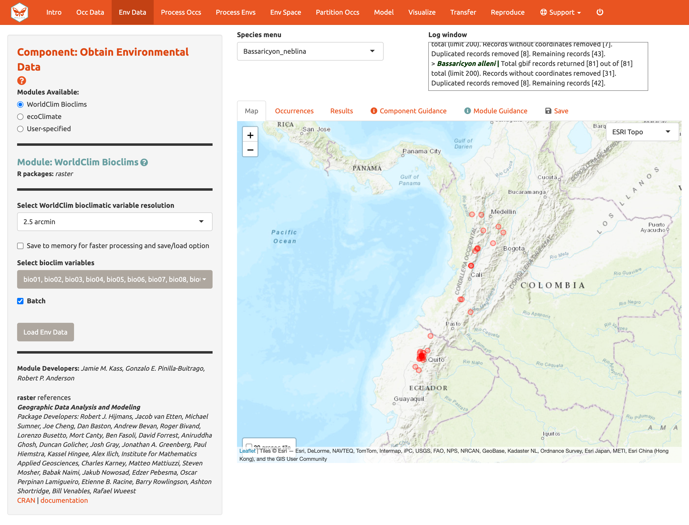
Although you could download the (very big) 30 arcsec global raster from the WorldClim website and load it into Wallace (preferably after cropping it with GIS software or in R), we will instead choose the 2.5 arcmin bioclimatic variable resolution that Wallace serves in a global extent to cover all our occurrence points, and we will keep all 19 bioclimatic variables checked. Note that the selections made will be performed only for the species selected in the Species Menu box, unless the “Batch” box is checked.

The “Batch” button will perform the analysis you’ve set up in the module for all the species you have uploaded. You’ll notice this option in many of the modules. If you want to perform individualized analyses for each species (in this case, different environmental variables), leave “Batch” unchecked. Note: The batch option is not available for 30 arcsec resolution since different tiles may need to be accessed.

Check Batch and Load Env Data.
Notice the progress bar in the bottom-right corner.

After the rasters have loaded, the “Results” tab will display summary information about them (e.g., resolution, extent, cell number, etc.). In addition to downloading the rasters, Wallace will also remove any occurrence points with no environmental values (i.e., points that did not overlap with grid cells with data in the rasters).

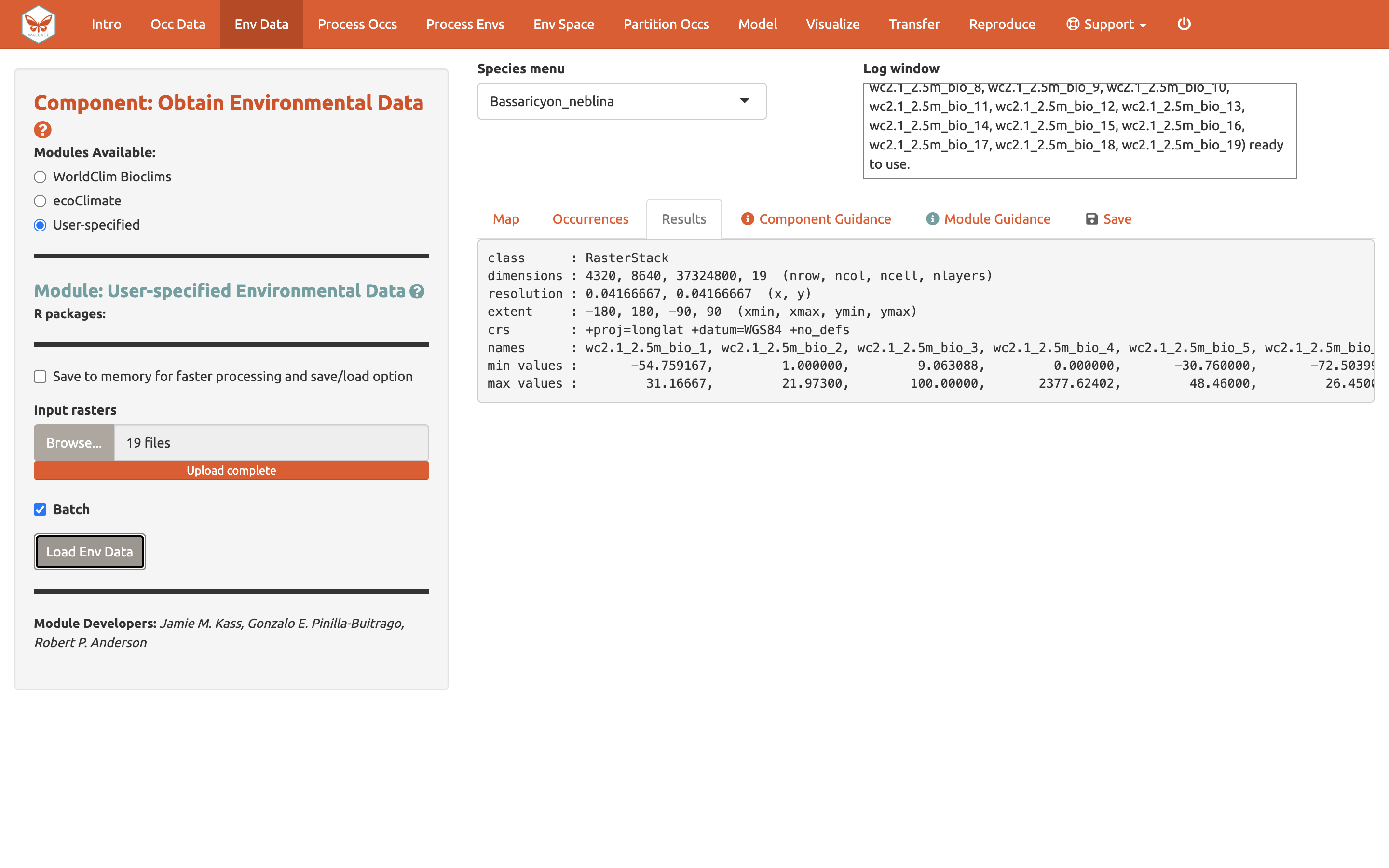
You can download your environmental variables from within the Download Data section of the “Save” tab.

Process Occurrence Data

The next component, Process Occs, gives you access to some data-cleaning tools. The data you retrieved from GBIF are raw, and there will almost always be some erroneous points. Some basic knowledge of the species’ range can help us remove the most obvious errors. For databases like GBIF that accumulate lots of data from various sources, there are inevitably some dubious localities. For example, coordinates might specify a museum location instead of those associated with the specimen, or the latitude and longitude might be inverted. In order to eliminate these obviously erroneous records, select only the points you want to keep for analysis with the module Select Occurrences On Map. Alternatively, you can also remove specific occurrences by ID with the module Remove Occurrences by ID. Even after removing problematic points, those you have left may be clustered due to sampling bias. This often leads to artifactually inflated spatial autocorrelation, which can bias the environmental signal for the occurrence data that the model will attempt to fit. For example, there might be clustering of points near cities because the data are mostly from citizen scientists who live in or near them. Or, the points can cluster around roads because the field biologists who took the data were either making observations while driving or gained access to sites from them. The last module, Spatial thin will help reduce the effects of sampling bias. Unlike other components, in Process Occs the modules are not exclusive, and all can be used in any order.

Make sure Bassaricyon alleni is in the species menu.
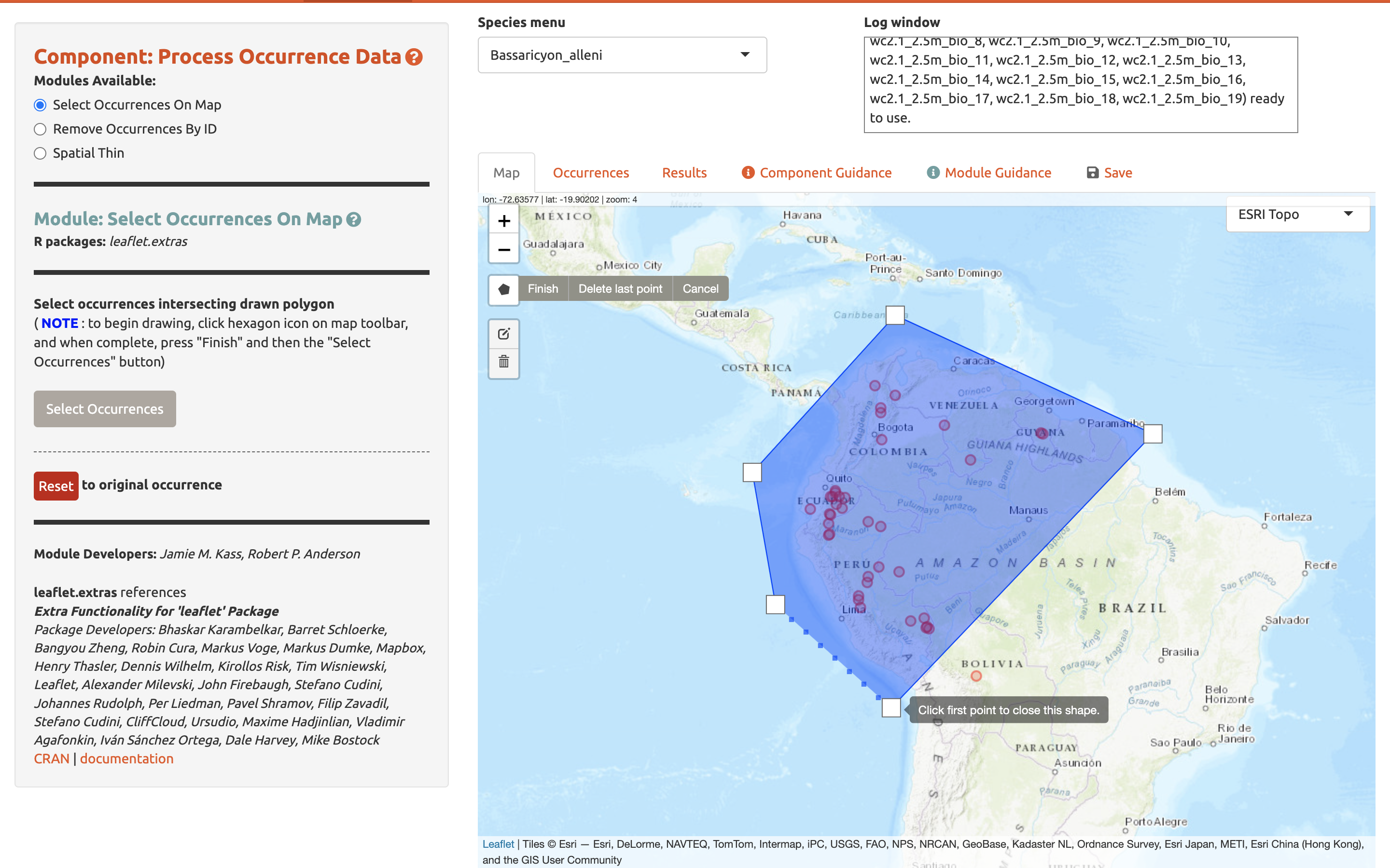
We will practice using the first two modules with this species. In the first module, we will use the polygon-drawing tool to select occurrences. The polygon drawing tool is useful to draw extents and will be seen in other modules later on as well.

Click on the polygon icon on the map toolbar.

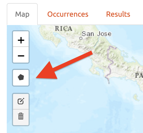
This opens the drawing tool. Click to begin drawing—each click connects to the last with a line. Draw a shape around South America, omitting the record in Bolivia. If you make a mistake in drawing, you can click “Delete last point” or “Cancel” to start over. To finish drawing, click again on the first point you made, or click “Finish” in the drawing tool. This finalizes the shape to use in analysis. Now click “Select Occurrences” and you will see the point in Bolivia disappear. To remove the blue shaded polygon, click on the trashcan icon on the map toolbar and hit “Clear All”. If you are displeased or have made an error, the red “Reset” button in the module interface will revert back to the original points. Since we arbitrarily removed the record in Bolivia, click reset to return to our original dataset.

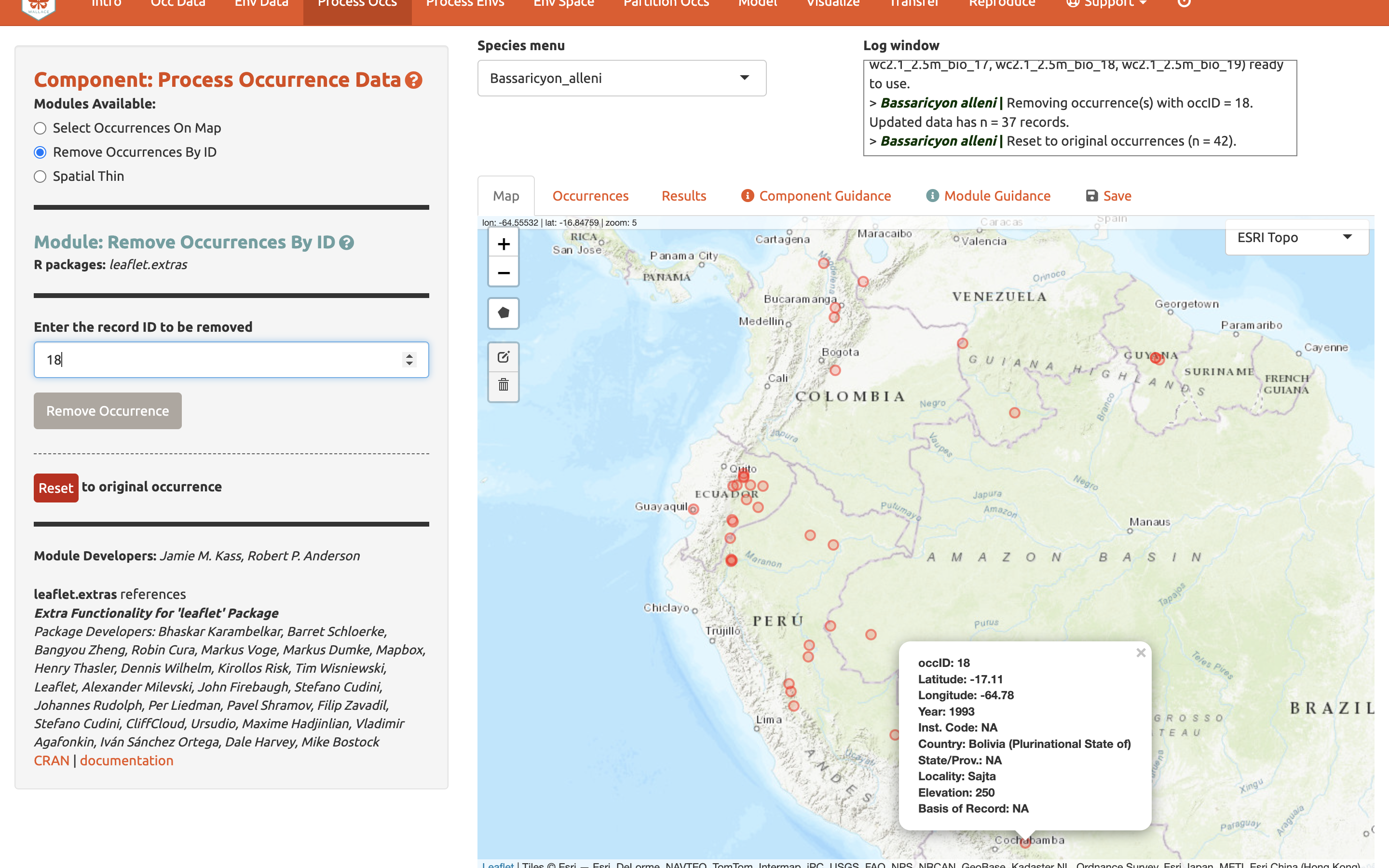
We will now remove it again, this time using the second module, Remove Occurrences by ID. With the pointer, click on the record in Bolivia. Information on the record will pop up, starting with the OccID. In this case it is OccID #18 (it may be a different number for you). Other information from the attribute table will be available. For example, the record has no information (NA) on the institution code, state/province, or basis. Since we know the OccID number, we can find the full information associated in the Occurrences tab. Click there and find the record. Here we can see it is a preserved specimen from the Museum of Southwestern Biology (MSB). Go back to the map. Enter “18” for the ID to be removed and “Remove Occurrence”. You will see the point disappear again. Click reset to get it back again.

Next, click on the module Spatial Thin. This lets you attempt to reduce the effects of spatial sampling bias by running a thinning function on the points to filter out those less than a defined distance from one another. We will use “10 km” as an example and thin for each species separately by using the “Batch” option again.

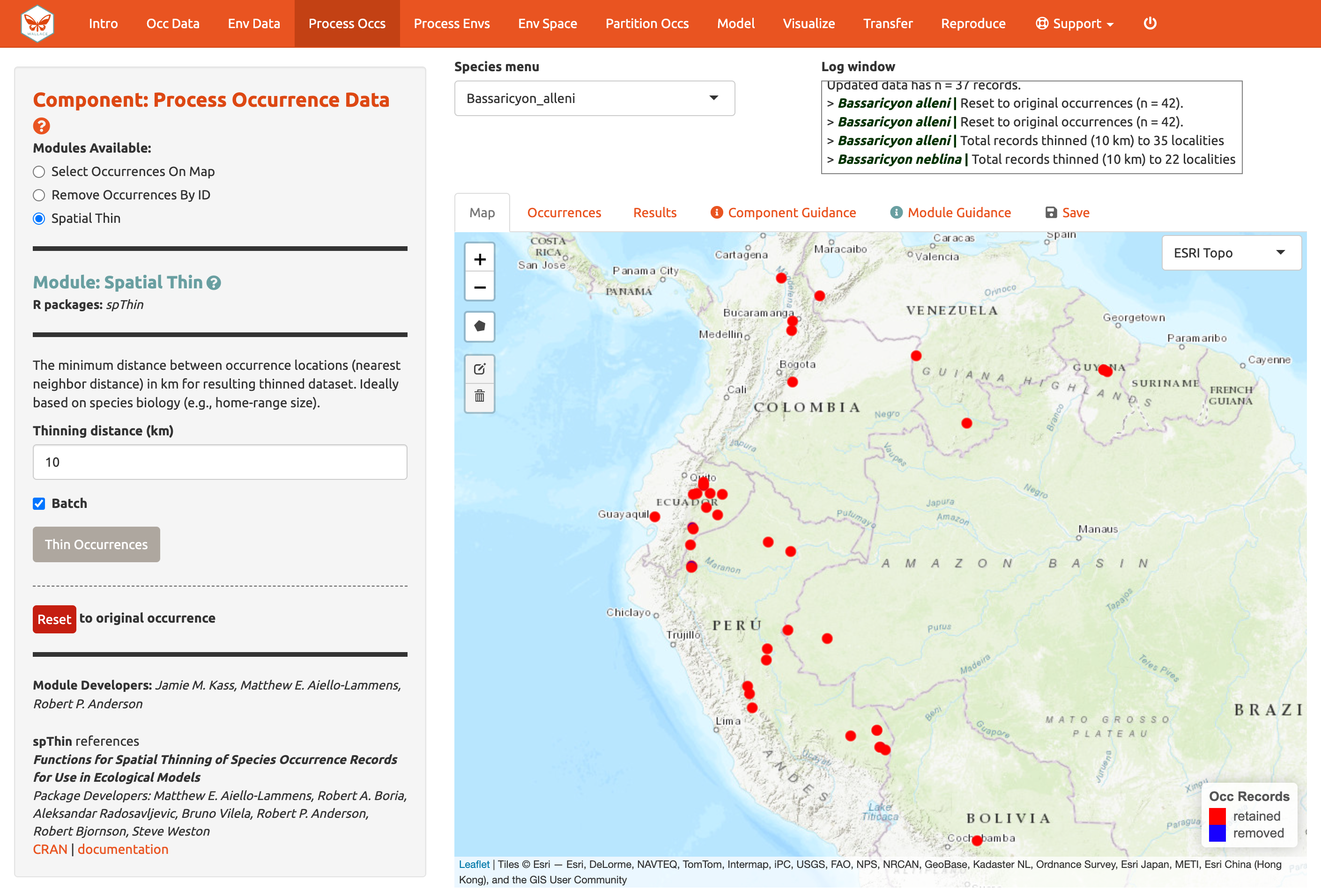
We are now left with 35 points for Bassaricyon alleni and 21 for Bassaricyon neblina (your numbers may be different). You can zoom in to see what the function did. Red points were retained and blue ones were removed. Download the processed occurrence datasets as a .csv file by clicking on the button in the “Save” tab. Reminder: the data downloaded are only for the species currently in the species menu.

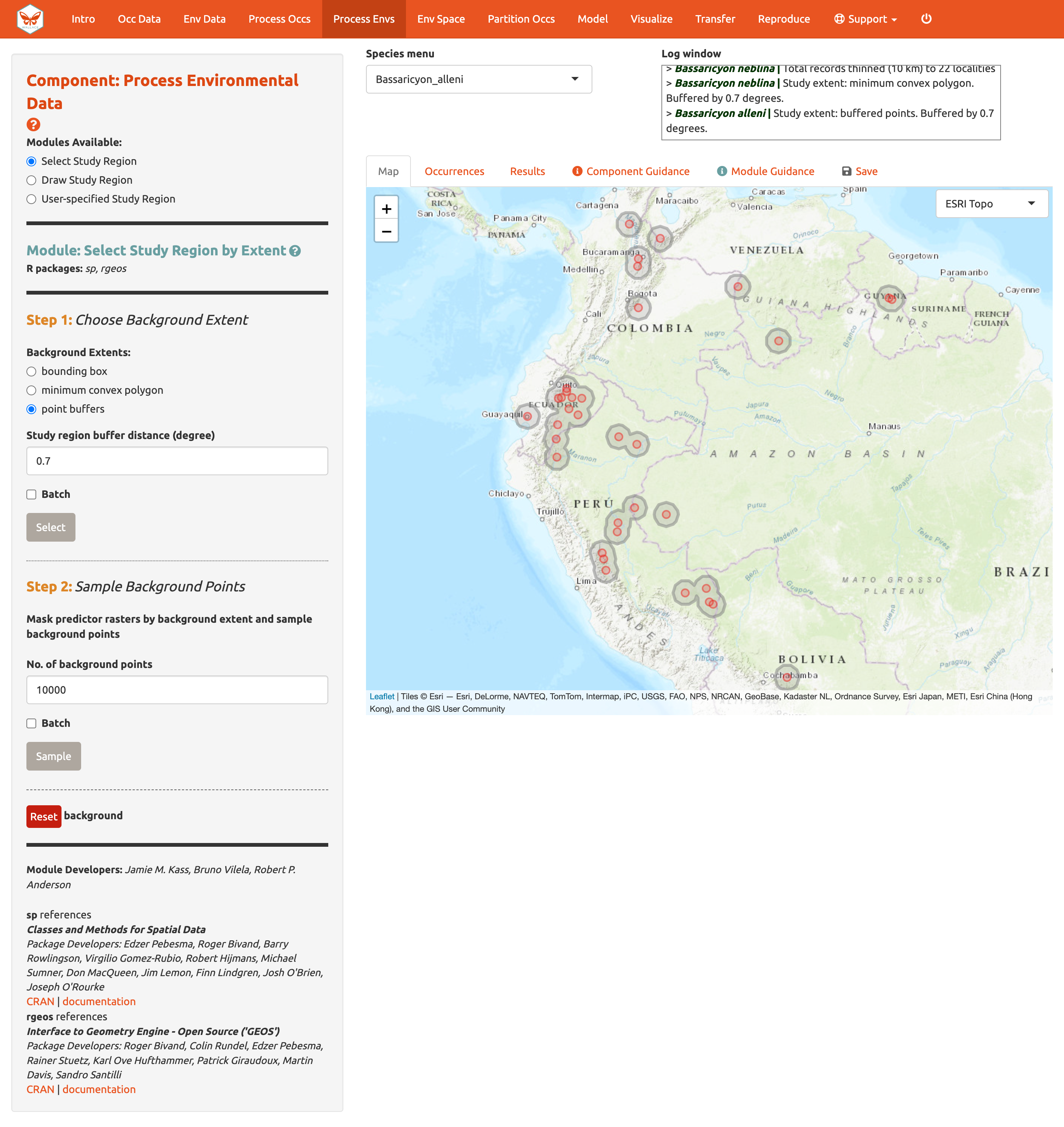
Process Environmental Data

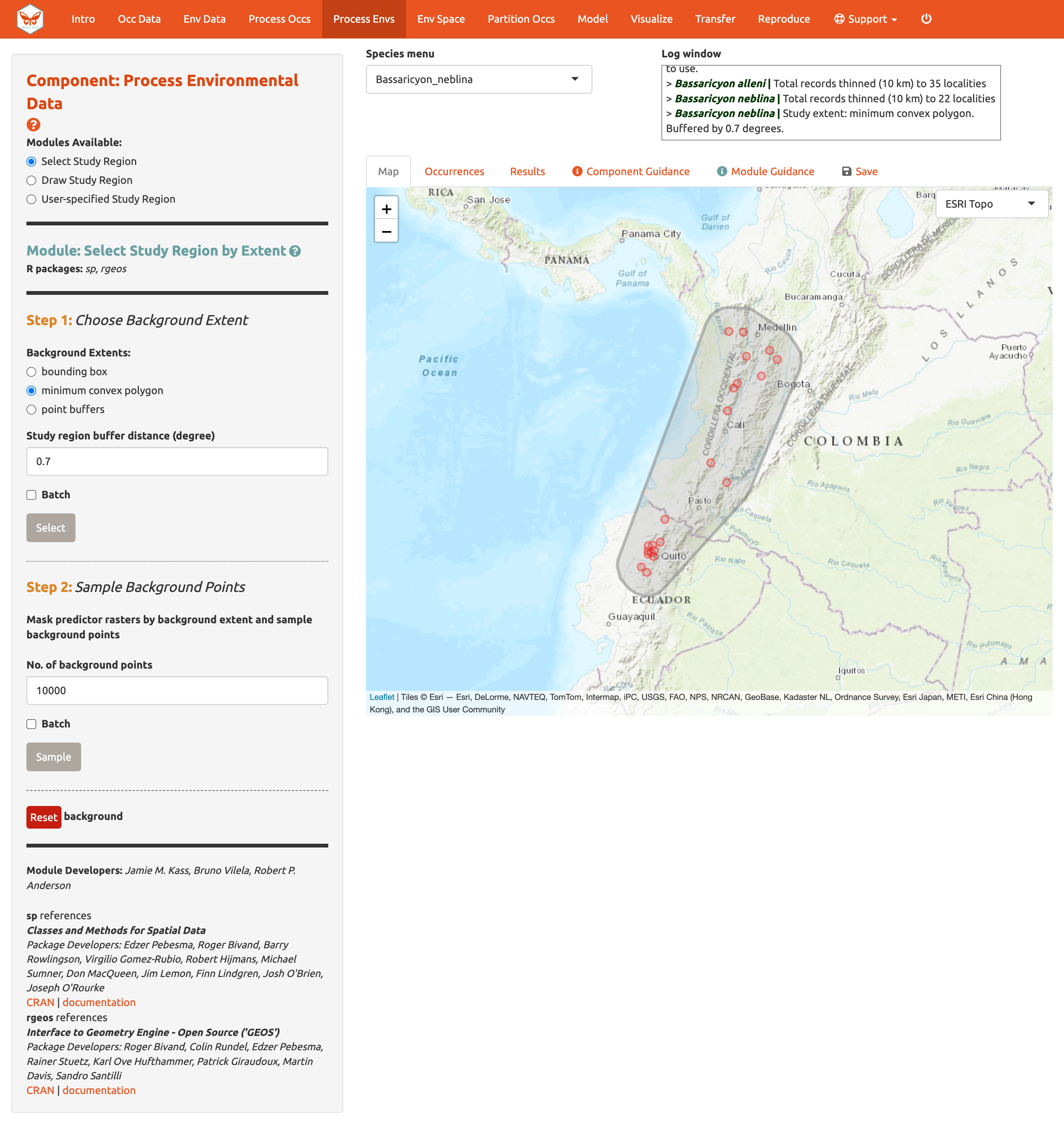
Now we will need to choose the study extent for modeling. This will define the region from which “background” points are drawn for model fitting. Background points are meant to sample the environments in the total area available to the study species. Methods like Maxent are known as presence-background techniques because they compare the predictor variable values at background points to those at the occurrence points (as opposed to presence-absence techniques, which require absence data). In making decisions about the study extent, we want to avoid areas the species has historically been unable to move to—for example, regions beyond a barrier like a mountain range or large river that the species cannot cross. Including these areas may send a false signal to the model that these areas are not environmentally suitable. Like every other step of the analysis, please see the relevant guidance text for more details.

You can explore the different options for delineating the study extent here. Each module has two steps: 1) choosing the shape of the background extent, and 2) sampling the background points. To begin, go to the module Select Study Region. Under “Step 1”, try out the different options and see how each one draws the background shape. Try increasing and decreasing the buffer to see how the shape is affected. Now set the species to B. neblina and use Select study region to a minimum convex polygon with a 0.7° buffer distance. Then switch to B. alleni and use point buffers with a 0.7° buffer.

Alternatively, you can draw your own polygon (using the same polygon drawing tool we tested in Component: Process occs). If you have a file specifying the background extent, you can upload it with the User-specified Study Region module. This module can accept a shapefile (must include .shp, .shx, and .dbf files) or a .csv file of polygon vertex coordinates with the field order: longitude, latitude. Note that the polygon you draw or shape you upload needs to contain all the occurrence points.

Next, complete “Step 2”, which both clips the rasters by the study extent and samples the background points. Set the number of background points to 10,000 (larger samples can be appropriate for larger extents or those with finer resolution; see component guidance text), check “Batch”, and click the “Sample” button.

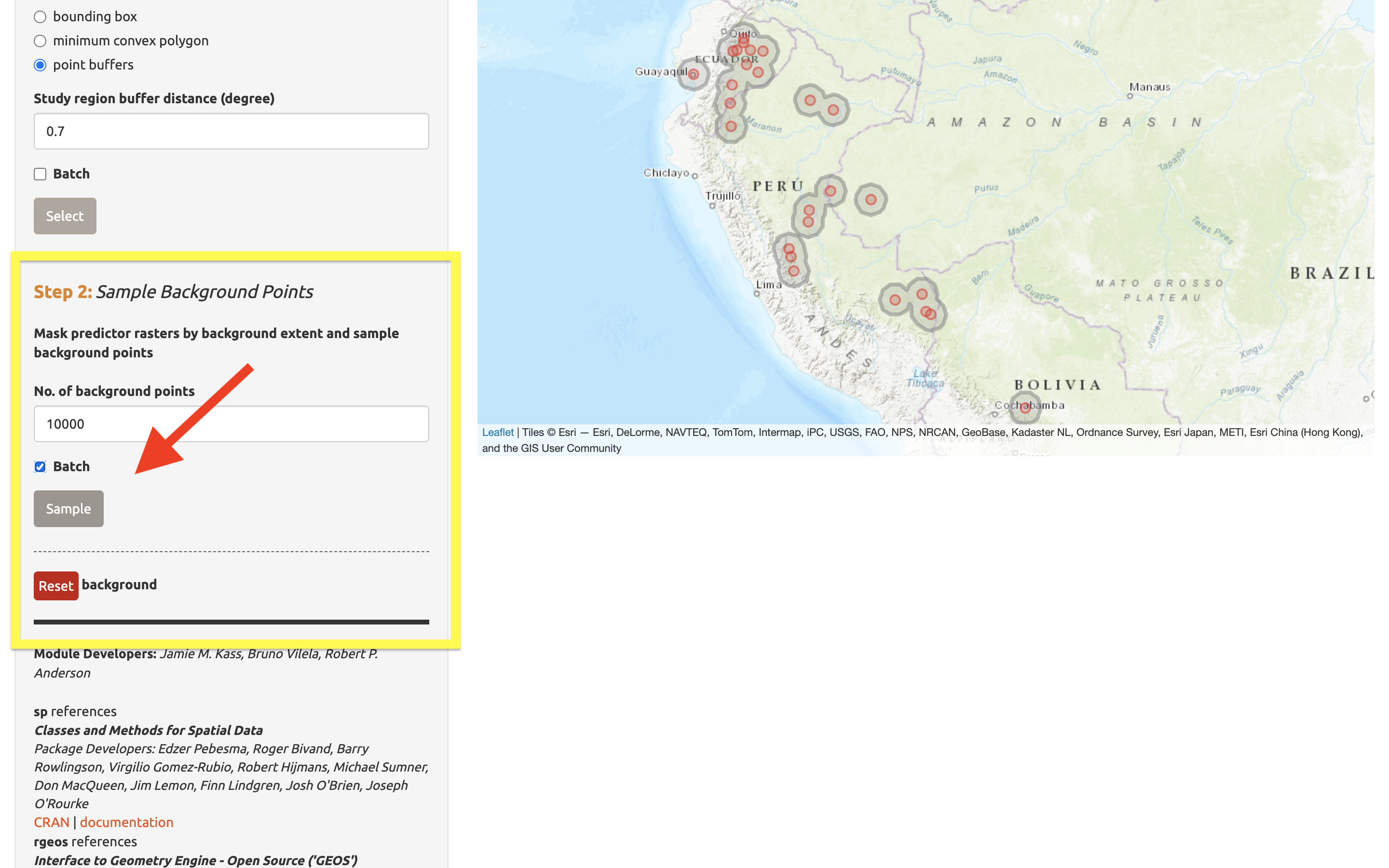
You may find that requesting 10,000 background points exceeds the number of grid cells in the background extent. The available number of points will be given in the log window, and that amount can be used instead of 10,000.

A .zip file of the clipped rasters (e.g., the environmental data clipped to the extent of the background you just created) is available to download in the “Save” tab. Make sure to toggle the species to download the file for each one.

Characterize Environmental Space

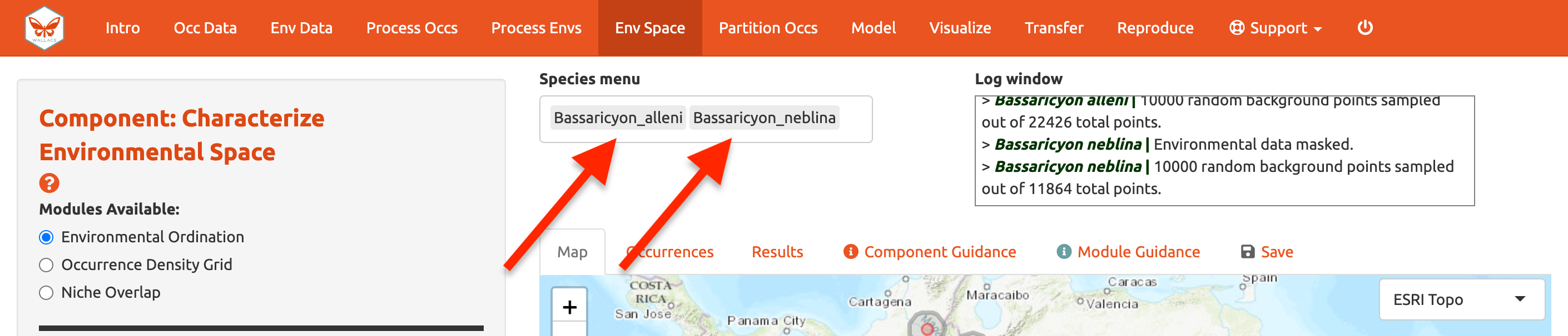
Component: Characterize Environmental Space contains multi-species analyses and is optional. Unlike some other components which let you perform the modules in any order, the modules within Characterize Environmental Space are sequential and thus need to be performed consecutively (i.e., you can’t get an Occurrence Density Grid without first performing an Environmental Ordination).

Before we begin the Module: Environmental Ordination analysis, you need to select two species to work with. If you had more than two species uploaded, select two from the species menu drop-down. Since we only have two uploaded, click in the species menu box and select the second species. Both names will appear in the box simultaneously—this functionality is currently only available for the Characterize Environmental Space component.

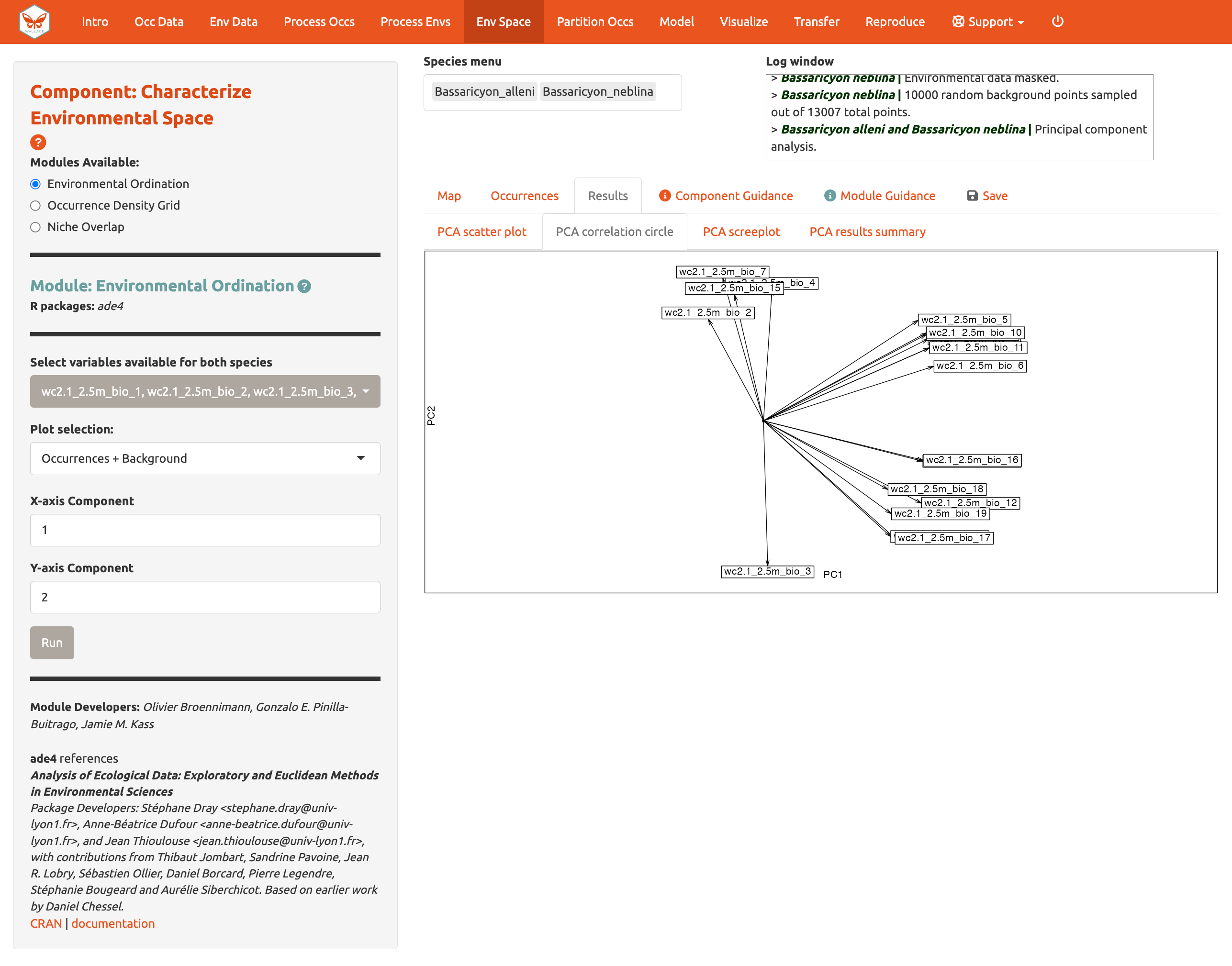
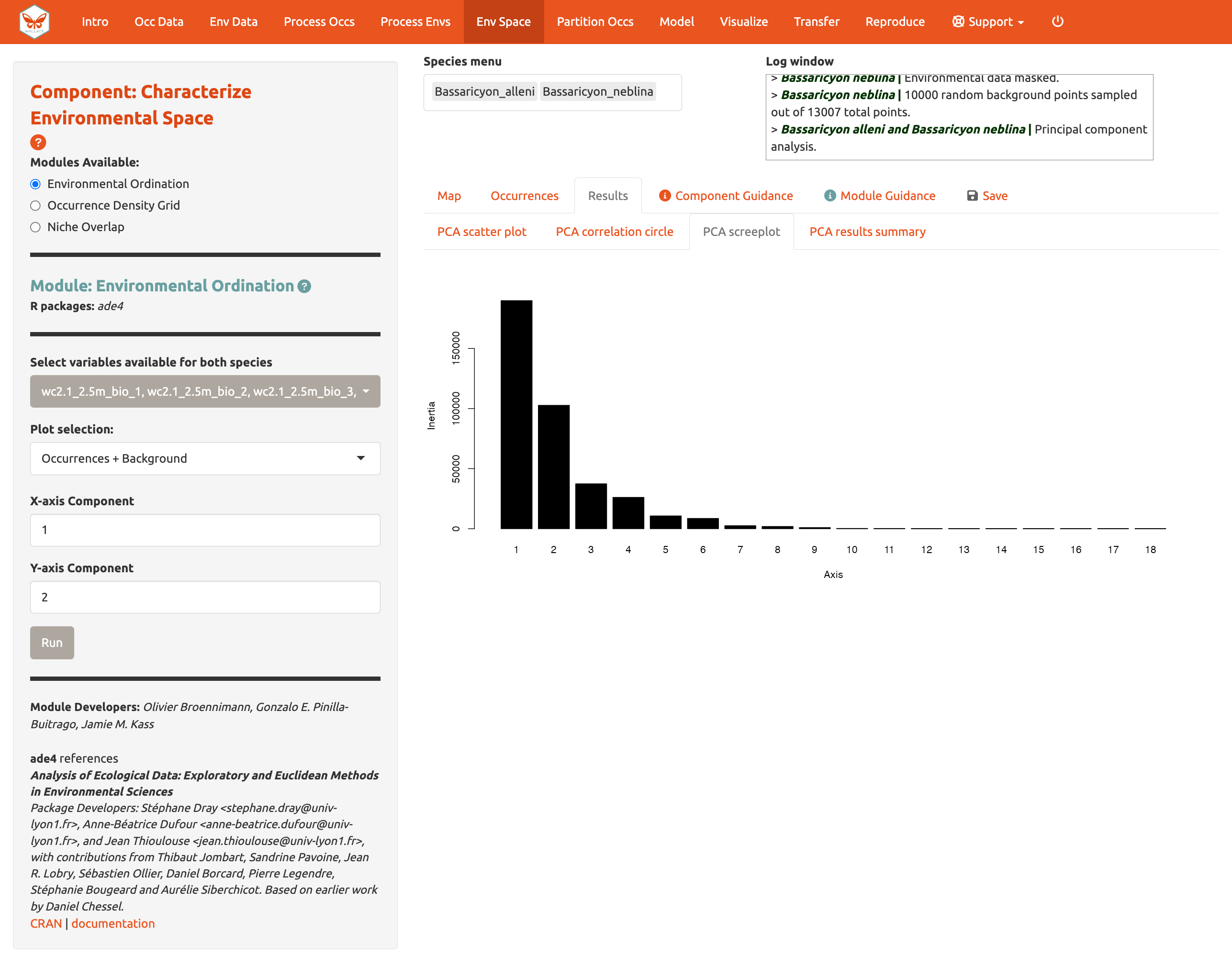
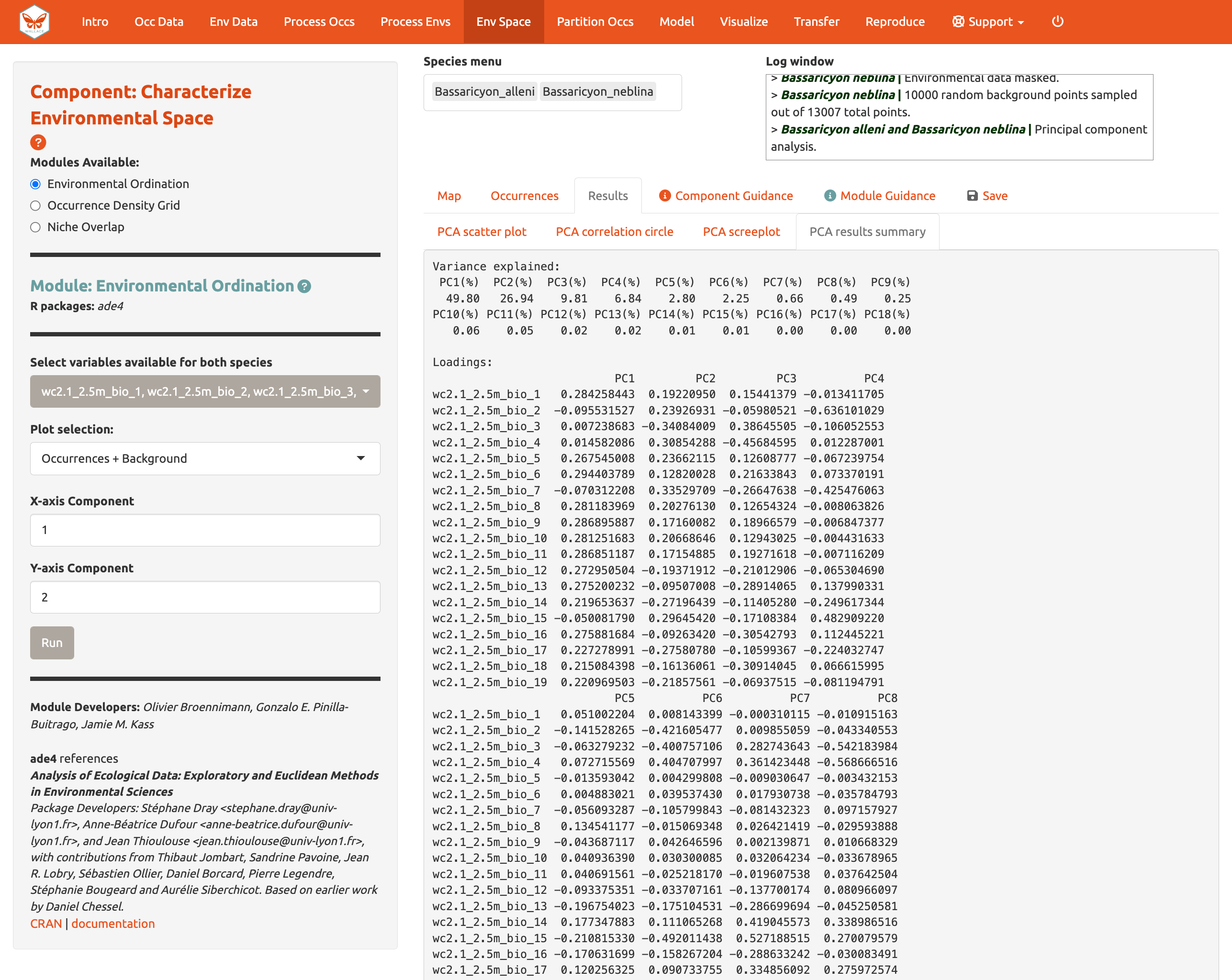
Module: Environmental Ordination is for conducting an ordination approach called Principal Component Analysis (PCA), that maximizes the variation contained in the predictor variables into fewer ones. To perform a PCA, select the variables available for both species by checking/unchecking the bioclimatic variables. Choose between “Occurrences Only” or “Occurrences & Background” for the plot selection and set the x- and y-axis components. The PCA Scatter Plot appears in the Results tab.

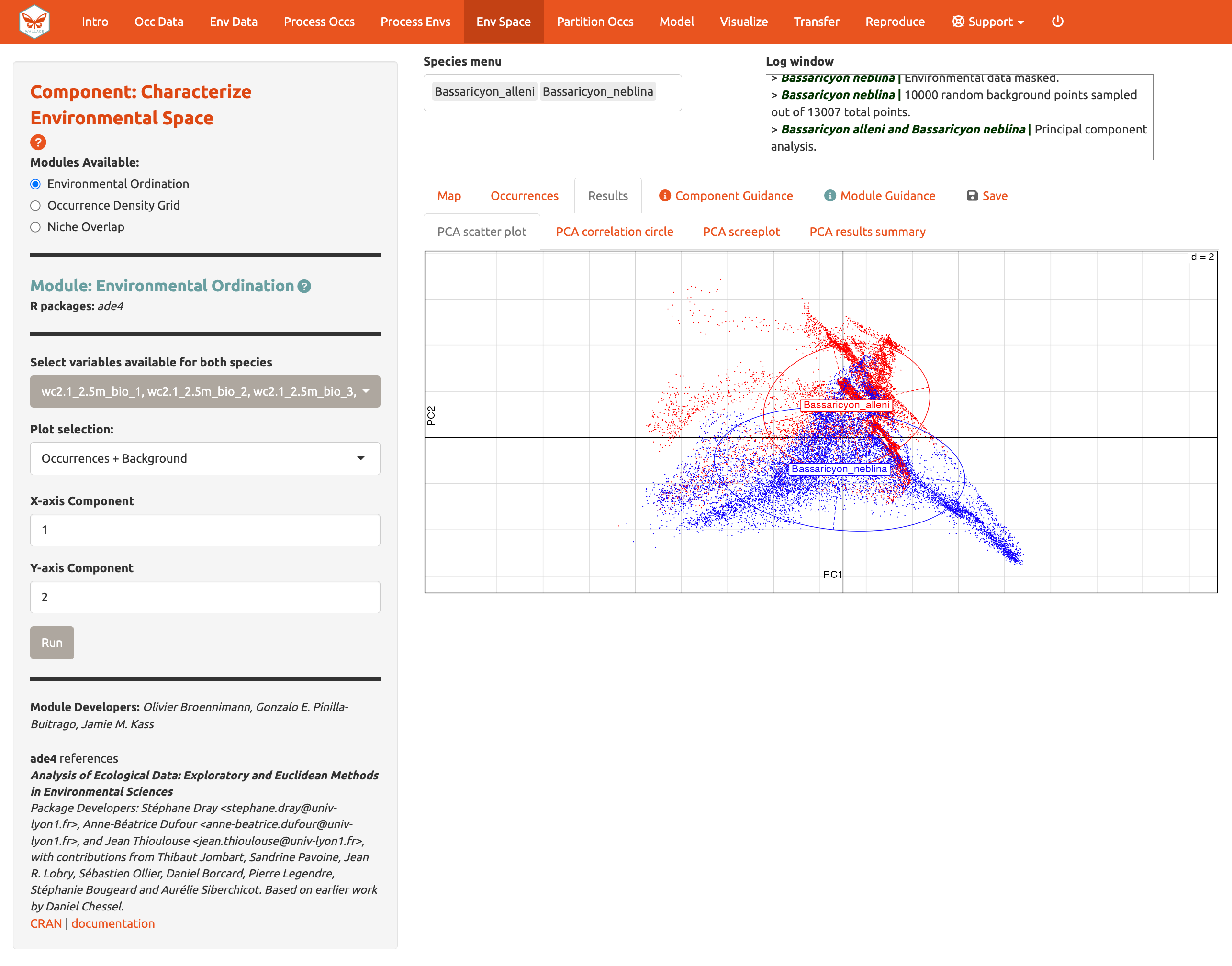
You can also view the PCA correlation circle, PCA scree plot, and the PCA results summary. For more information on these statistics and how to evaluate the results, consult the module guidance text.

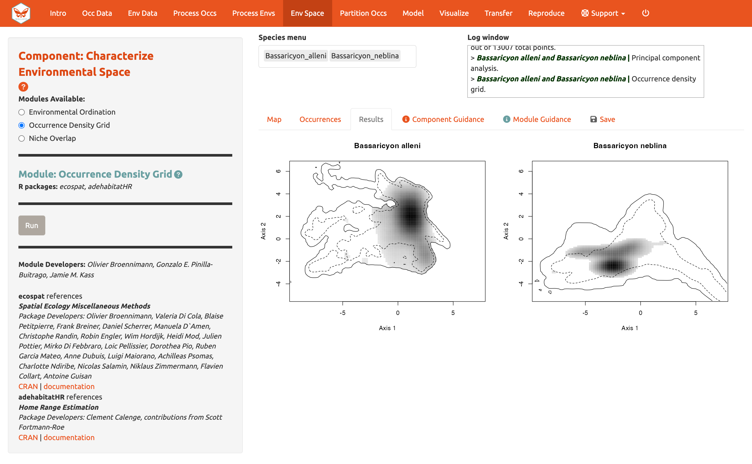
Next, run an Occurrence Density Grid. This calculates and plots which part of the environmental space is occupied more densely by the species and the availability of environmental conditions present within the background extent. Darker areas represent higher occurrence density. Areas within solid lines represent all environmental conditions available in the background extent, and areas within dashed lines represent the 50% most frequent ones

And calculate Niche overlap…

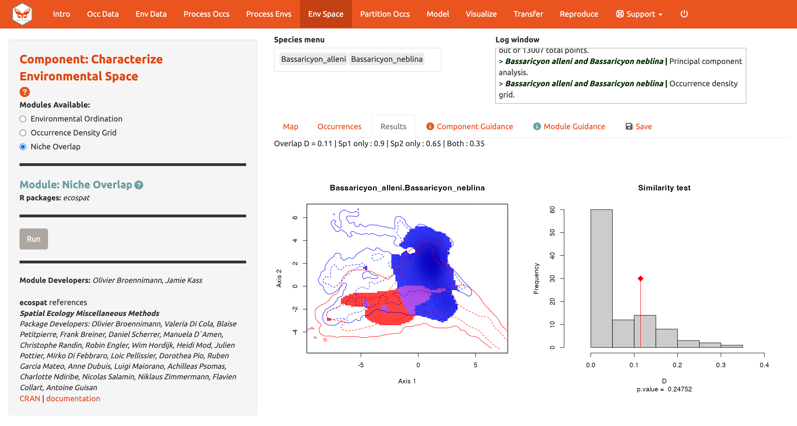
The niche overlap quantification is based on the occurrence and background densities in the available environmental space estimated in Module: Occurrence Density Grid. The overlap is quantified using Schoener’s D metric. The environmental conditions covered only by the niche of species 1 are shown in blue, the environmental conditions covered only by the niche of species 2 are shown in red, and the environmental conditions covered by both species, or the niche overlap, is shown in purple. In the Similarity Test, if the observed overlap (red line) is higher than 95% of the simulated overlaps (p-value < 0.05), we can consider the two species to be more similar than random, which is not what we see here. Again, consult the module guidance texts for more help to understand the analyses and help on evaluating the results.

Download the PCA results (.zip), density grid (.png), and overlap plot (.png) from the “Save” tab.

Partition Occurrences

We have not built any distribution models yet, but before we do, we will make decisions on how to partition our data for evaluation. In order to determine the strength of the model’s predictive ability, you theoretically need independent data to test it. When no independent datasets exist, one solution is to partition your data into subsets that we assume are independent of each other, then sequentially build a model on all the subsets but one and evaluate the performance of this model on the left-out subset. This is known as k-fold cross-validation (where k is the total number of subsets, or ‘folds’), which is quite prevalent in statistics, especially the fields of machine learning and data science. After this sequential model-building exercise is complete, Wallace averages the model performance statistics over all the itinerations and then builds a model using all the data.

There is a whole literature on how to best partition data for evaluating models. One option is to simply partition randomly, but with spatial data we run the risk that the groups are not spatially independent of each other. The jackknife method (“leave-one-out”) is recommended for species with small sample sizes and has previously been used for modeling Bassaricyon neblina (Gerstner et al. 2018) but may have long computational times.

Another option is to partition spatially—for example, by drawing lines on a map to divide the data. Spatial partitioning with k-fold cross-validation forces the model to predict into regions that are distant from those used to train the model (note that Wallace also excludes background points from regions corresponding to the withheld partition). For Bassaricyon alleni, environmental conditions in Colombia and Ecuador may differ considerably from conditions in Bolivia. If the model has accurate predictions on average on withheld spatially partitioned data, it likely has good transferability, which means it can transfer well to the new values of predictor variables (because distant areas are usually more environmentally different than close ones). As always, please refer to the guidance text for more details on all the types of partitioning offered in Wallace.
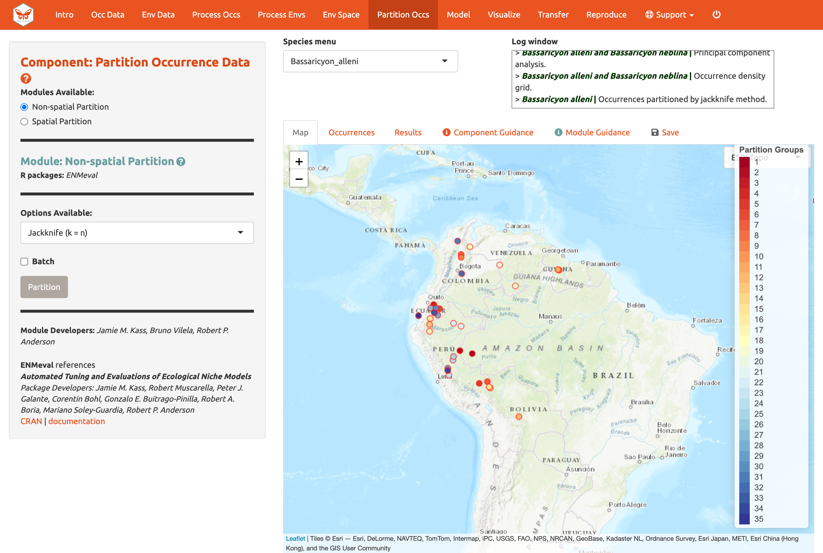
Here’s an example of jacknife (k = n), which assigns each point to its own partition group, so the number of bins equals the number of occurrences.

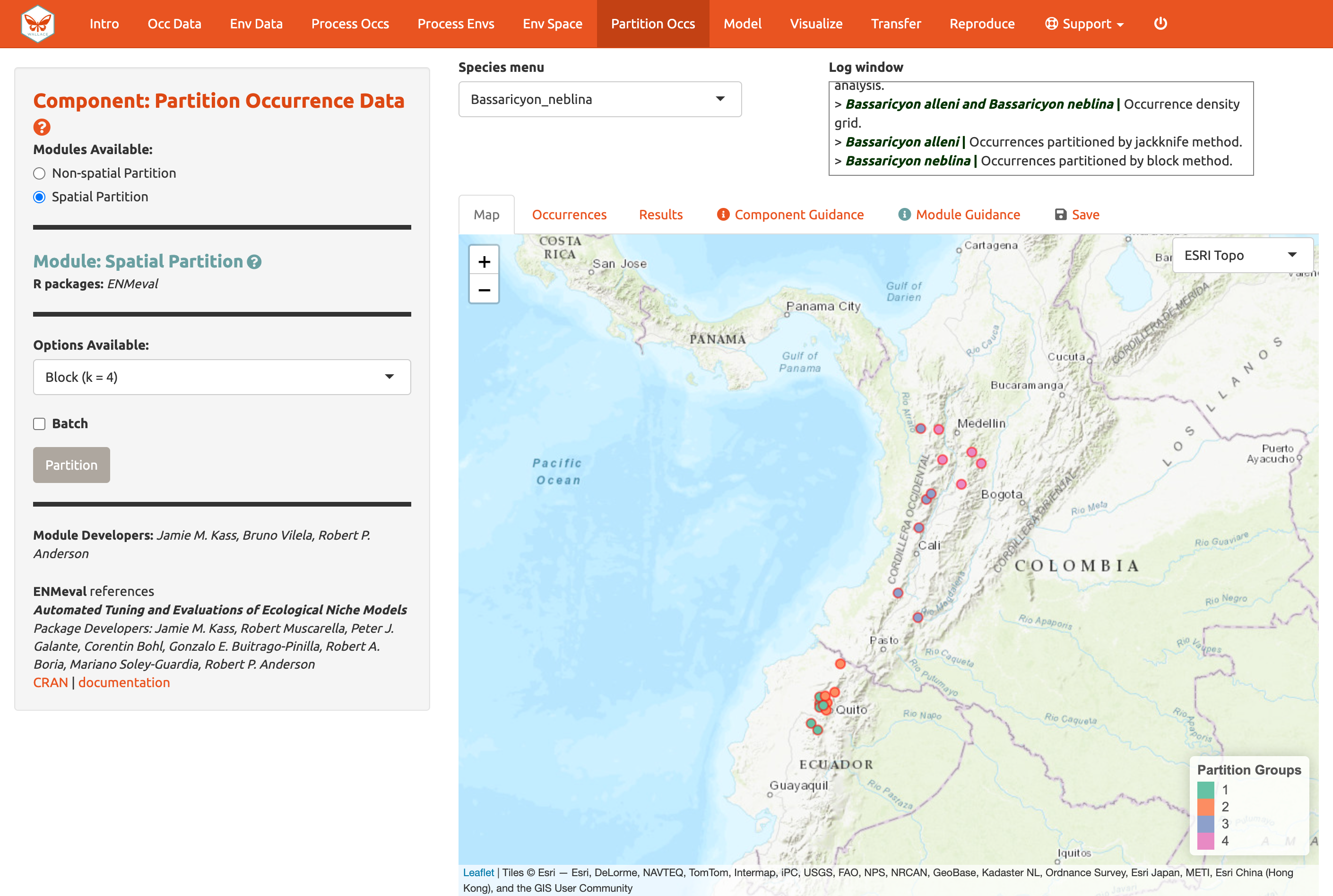
Now here is an example of spatial blocking, which assigns each point to one of four spatially separate partition groups.

We’ll use this last method now for faster computation, but it is recommended to review the guidance text and other literature––and talk to your peers!—to make an informed decision on partition methods.

Partition both species using Module: Spatial Partition Block (k = 4) option.

Save & Load Session

Before we go into Modeling, let’s explore one of the great features of Wallace v2, which is the ability to stop and save your progress to be continued later. If you want to skip this step (and risk losing everything if an error occurs except the data or results you have downloaded), you can move on to Model.

Click ‘Save Session’ within the “Save” tab. This tab is available from any of the Components. This will save your progress as an RDS (.rds) file, a file type used to save R objects. After it is saved, you can hit the stop sign in the upper right corner or close the browser window and exit R/RStudio. Note: if the Wallace session is closed before saving results and/or the session, all work will be lost.

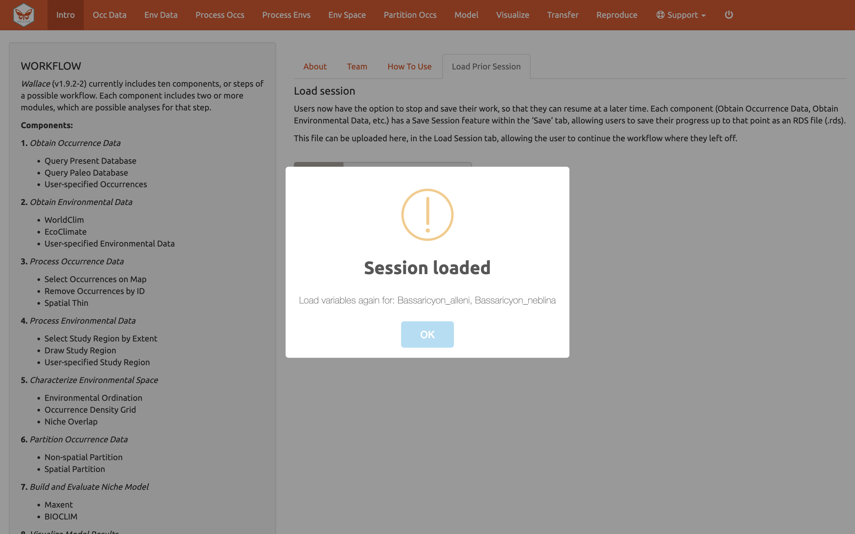
When you are ready to resume, load Wallace again.

library(wallace)
run_wallace()

In the Intro component, use the “Load Prior Session” tab to import your .rds session file.

A box will pop up– It looks like other Wallace warning messages, but in this case it is indicating the session is loaded. It may be necessary to reload your variables, using Occ Data and Env Data as previously carried out. You can now carry on with the previous analysis.

Model

We are now ready to build a distribution model. Wallace v2.0 provides two algorithm options; Maxent and BIOCLIM. For this vignette, we’ll use Maxent, a machine learning method that can fit a range of functions to patterns in the data, from simple (i.e., straight lines) to complex (i.e., curvy or with lines that can change direction; these can get jagged if complexity is not controlled). For more details on Maxent, please consult the Maxent website abnd guidance text.
Maxent is available to run through maxnet package or through Java with the maxent.jar option. In the interest of time and to avoid Java-related issues, let’s choose the following modeling options:

Choose maxnet
Select L, LQ, and H feature classes. These are the shapes that can be fit to the data:
- L = Linear, e.g. temp + precip
- Q = Quadratic, e.g. temp^2 + precip^2
- H = Hinge, e.g. piecewise linear functions, like splines (think of a series of lines that are connected together)
Select regularization multipliers between 0.5 and 4 with a step value of 0.5.
- Regularization is a penalty on model complexity.
- Higher values = smoother, less complex models. Basically, all predictor variable coefficients are shrunk progressively until some reach 0, when they drop out of the model. Only those variables with the greatest predictive contribution remain in the model.
Keep “NO” selected for categorical variables. This option is to indicate if any of your predictor variables are categorical, like soil or vegetation classes.
- Had you loaded categorical variables, you would check here and then indicate which of the rasters is categorical.
Set Clamping? to “TRUE”. This will clamp the model predictions (i.e., keep the environmental values more extreme than those present in the background data to within the bounds of the background data).
If you set Parallel? to “TRUE”, you can indicate the number of cores for parallel processing.

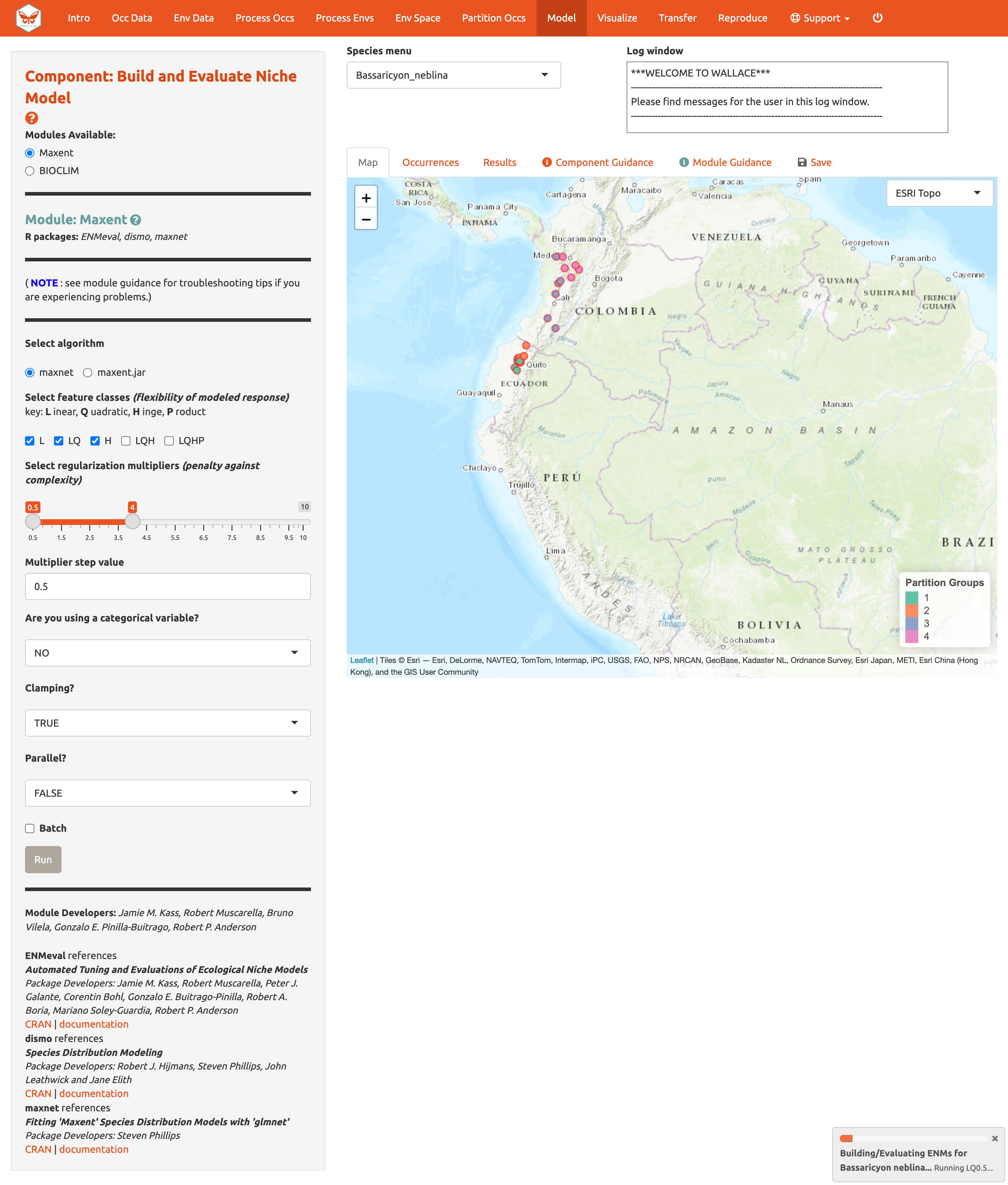
We will construct a model for Bassaricyon neblina, but note that the Batch feature can be checked to run these selections for all species you have uploaded.
Make sure Bassaricyon neblina is selected in the species menu and Batch is unchecked before hitting Run.

The 3 feature class combinations (L, LQ, H) x 8 regularization multipliers (0.5, 1, 1.5, 2, 2.5, 3, 3.5, 4) = 24 candidate models. The hinge feature class (H) will enable substantial complexity in the response, so it takes a bit longer to run than the simpler models.

The results appear in two tables of evaluation statistics, allowing comparison of the different models you just built. The first table shows the statistics for the full model and partition averages. There should be 24 rows: one for each of the feature class / regularization multiplier combinations. In the first table, statistics from the models built from the 4 occurrence data partition groups (one withheld for each iteration) are averaged. In the second table, the partition group statistics averaged in the first table are shown, and thus it contains 96 rows (each of the 4 folds for each of the 24 models).

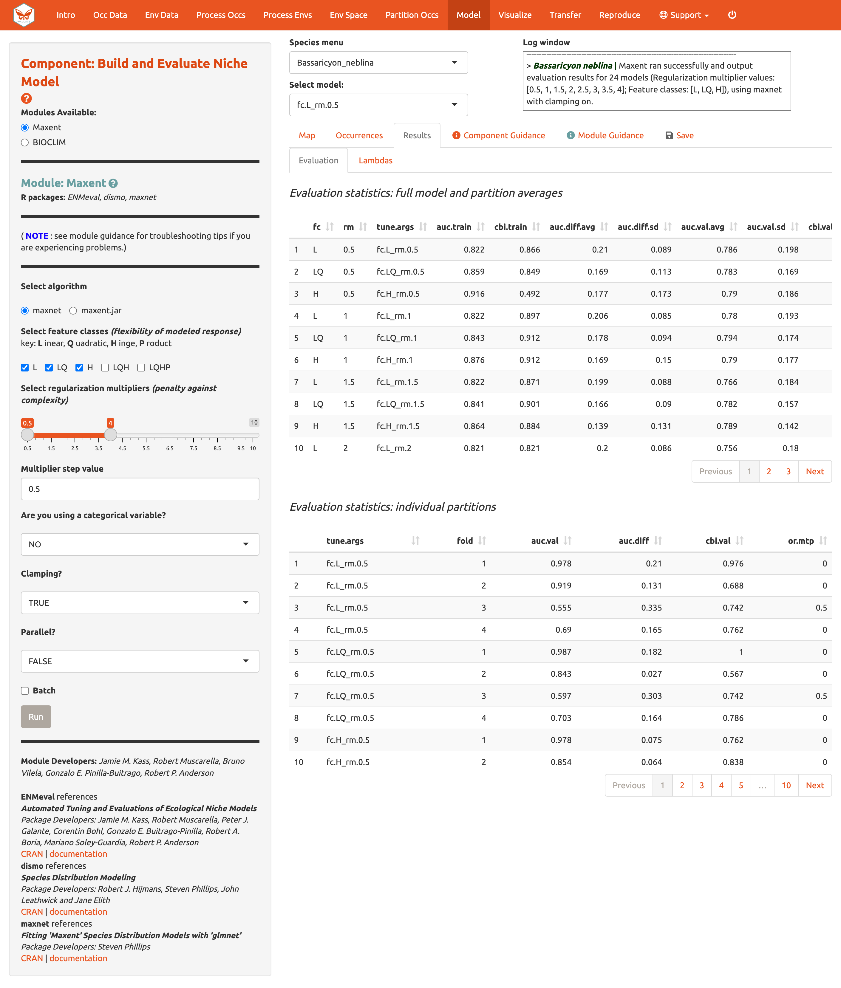
How do we choose the “best” model?
There is a mountain of literature about this, and there is really no single answer for all datasets. The model performance statistics AUC (Area Under the Curve), OR (Omission Rate), and CBI (Continuous Boyce Index) were calculated and averaged across our partitions, and AICc (corrected Akaike information criterion) was instead calculated using the model prediction of the full background extent (and all of the thinned occurrence points). Although AICc does not incorporate the cross-validation results, it does explicitly penalize model complexity—hence, models with more parameters tend to have a worse AICc score. It’s really up to the user to decide, and the guidance text has some references which should help you learn more.

The evaluation metrics table can be sorted. First, we will prioritize models that omitted few occurrence points in the predicted area during cross-validation. Sort the results table in ascending order by “or.10p.avg”, or the average omission rate when applying a 10-percentile training presence threshold to the (withheld) validation data (see guidance text for details). As we would prefer a model that does not omit many withheld occurrences when it makes a range prediction, we are prioritizing low values of “or.10p.avg”.

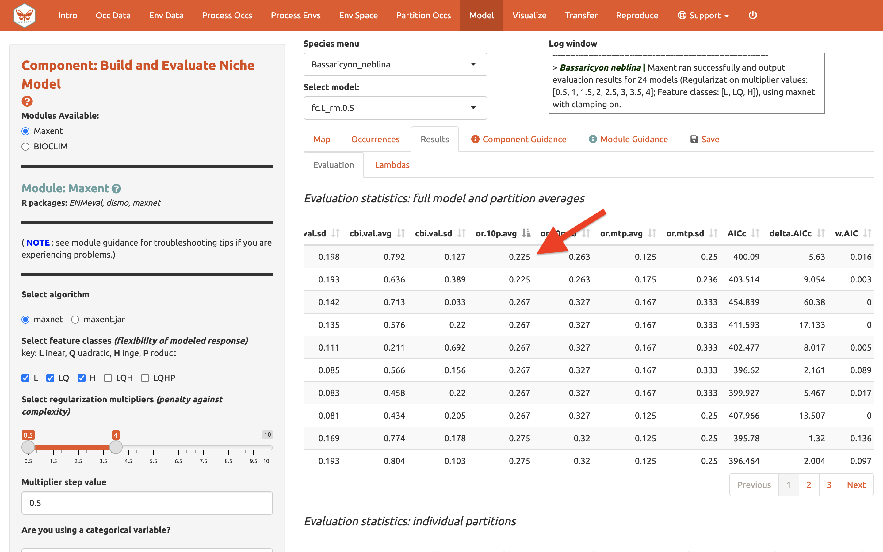
Let’s also look at average validation AUC values (where higher values are better).

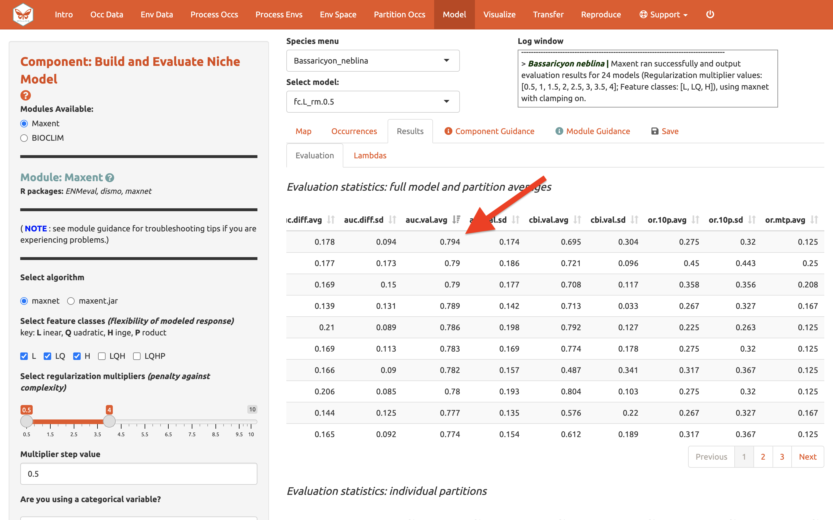
And AICc (where lower values are better)…

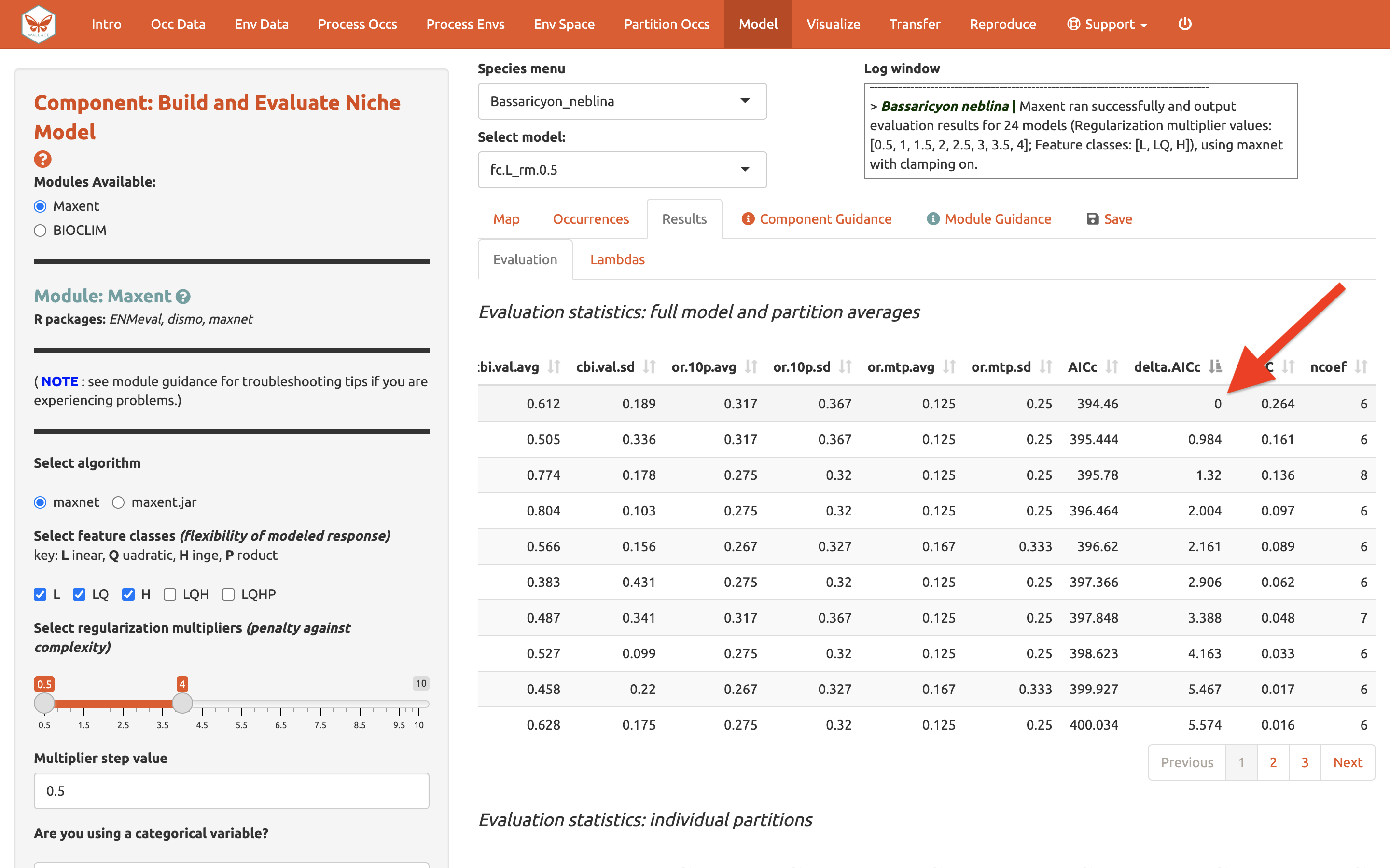
In our example, if we had chosen the model with the lowest AICc score, we would have ended up with LQ_2. Note: your values may be different.

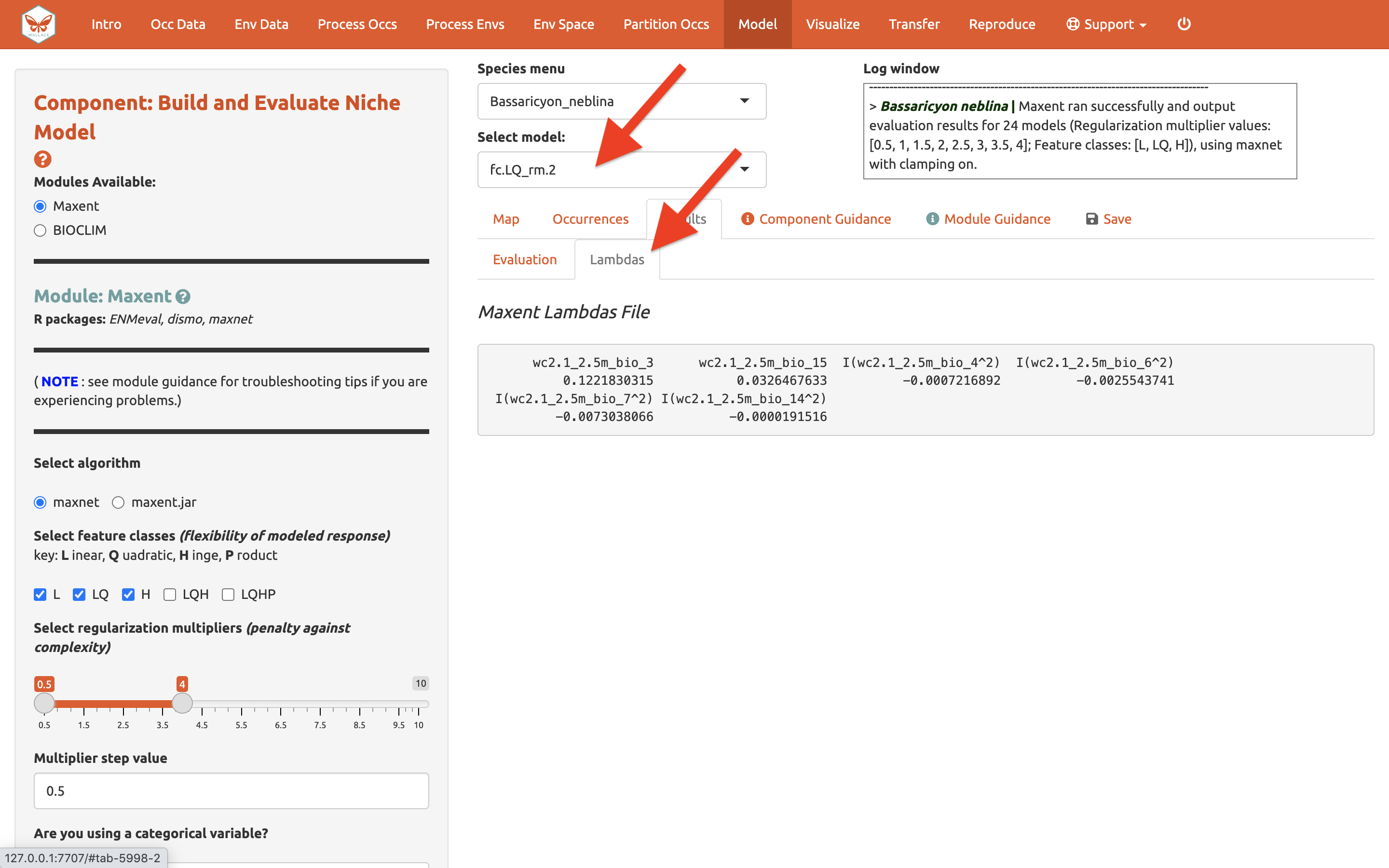
Next to the Evaluation results, you can access the Maxent Lambdas file (which describe the weights for feature classes of each variable) for each of the models (changing the candidate model in the drop-down box changes the output).

Use the “Save” tab to download the evaluation tables.

Visualize

There are four modules for Visualization. We’ll save the first, Map Prediction, for last. We’ll skip the fourth module, BIOCLIM Envelope Plot, since we used Maxent instead of BIOCLIM.
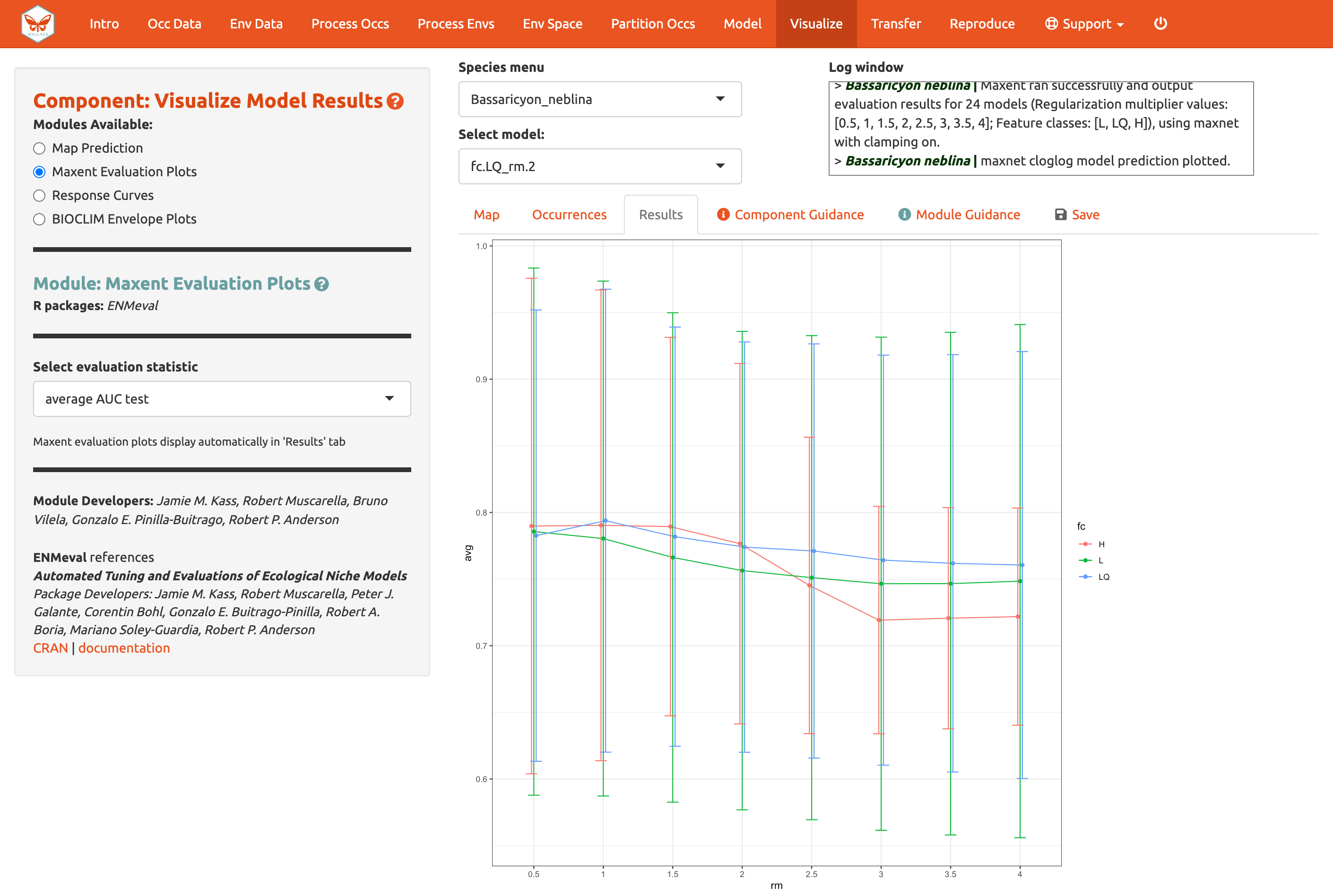
The module Maxent Evaluation Plots, enables users to evaluate the performance statistics across models. Graphs appear in the Results tab. Below, see how the feature class and regularization multiplier selections affect average validation AUC values.

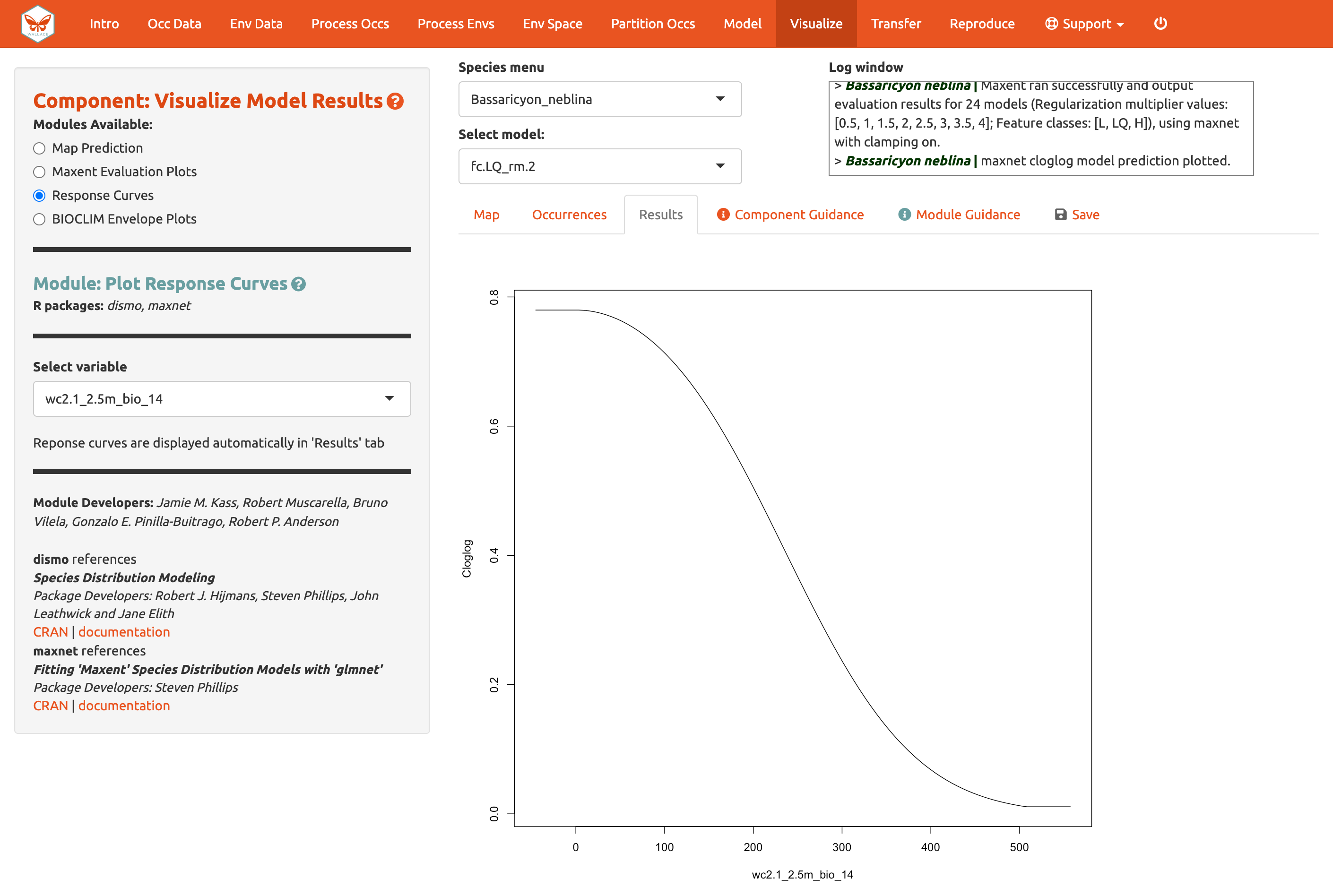
We should also examine the response curves, which show how the predicted suitability (y-axis) changes based on different values of each variable (x-axis). For these curves, the marginal response of one variable is shown while the other variables are held at their mean values. If you want to see the results for a particular model, select it by using the dropdown menu below the species box. Below is a response curve for model LQ_2 for the mean precipitation of the driest month (bio14).

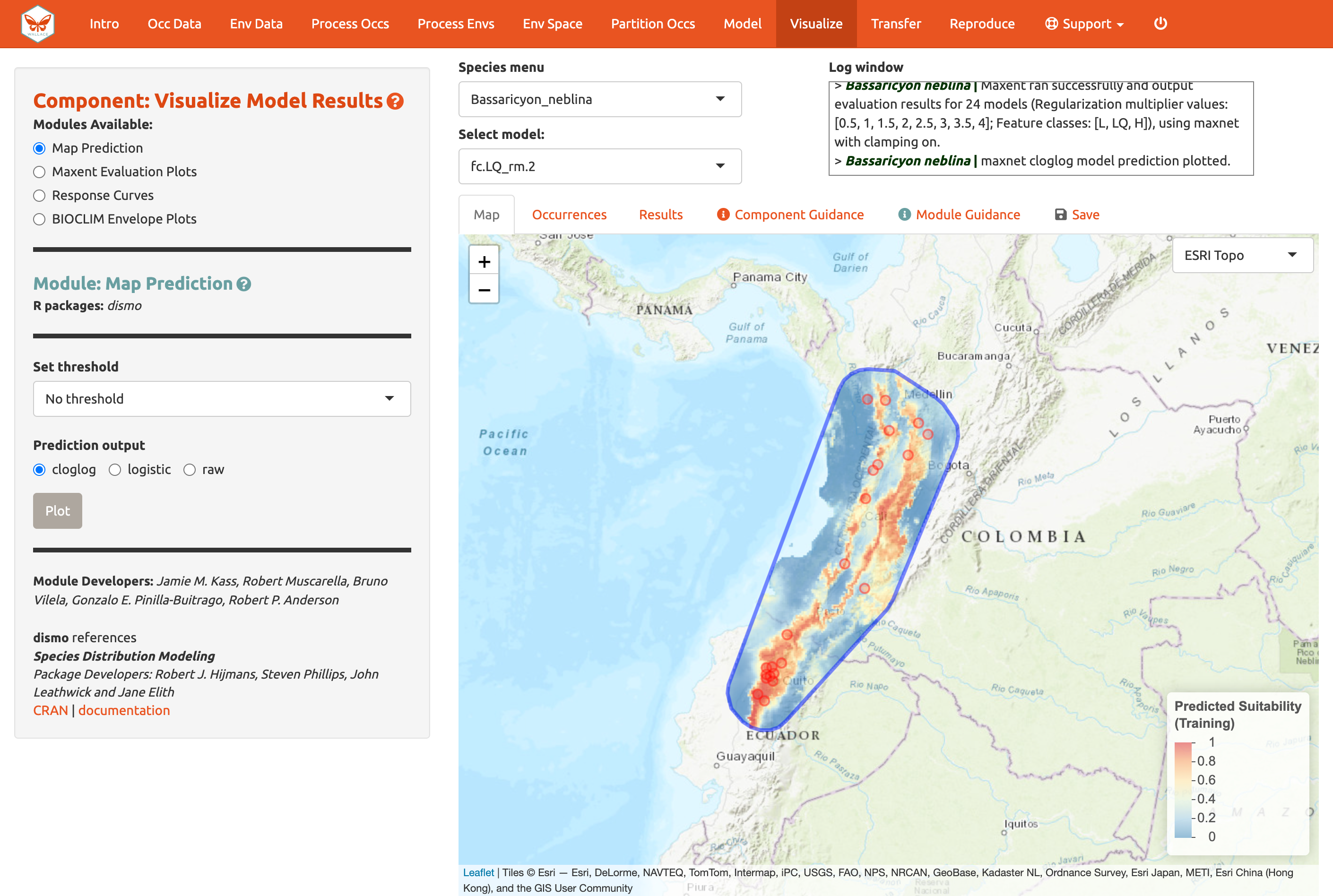
Of course, you can also visualize model predictions on the map. Predictions of suitability can be continuous (a range of values from low to high) or binary (thresholded to two values: 0, unsuitable and 1, suitable). We are visualizing predictions made with the “cloglog” transformation, which converts the raw Maxent output (relative occurrence rate) to a probabilistic scale between 0 and 1 to approximate probability of presence (given key assumptions). Please see the module guidance for information about Maxent model output scalings and thresholding rules. Here is the mapped prediction for model LQ_2, no threshold, in cloglog output.

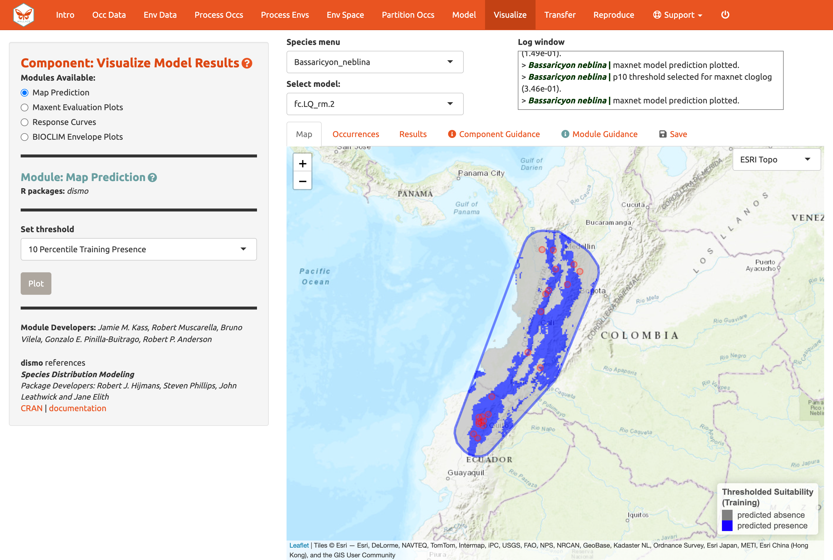
Below is the mapped prediction of the same model, this time with the threshold set to the 10-percentile training presence value (the occurrence suitability value we used to calculate omission rates above to help us select models). Some of the occurrence points will fall outside the blue regions that represent suitable areas for Bassaricyon neblina. For the 10-percentile training presence value, as it represents not the lowest predicted suitability, but the value greater than the 10% lowest, the expected omission would be 0.1 (i.e., 10% omitted).

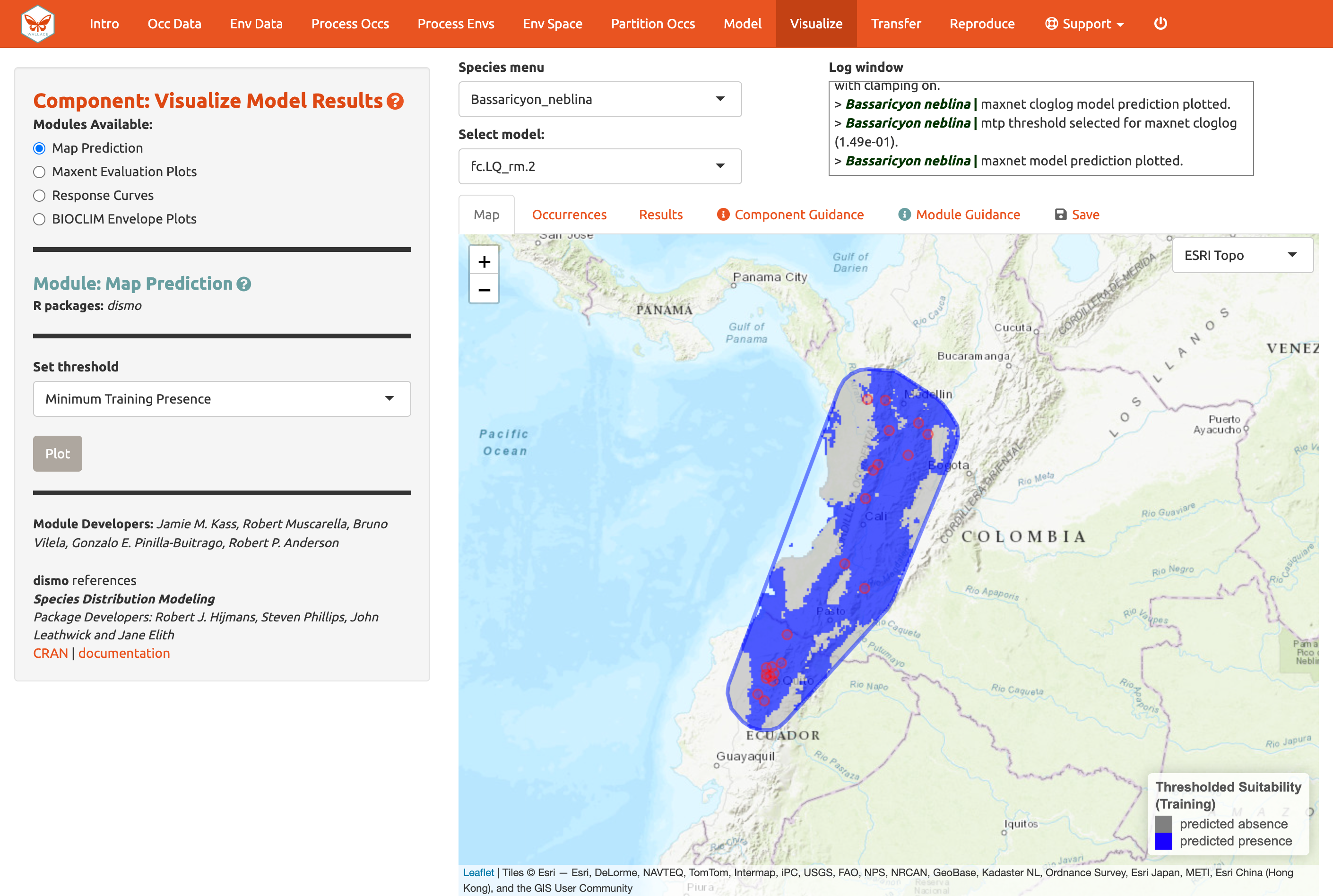
Try mapping the prediction with the threshold set to the less strict ‘minimum training presence’ and notice the difference. You can also threshold by a quantile of training presences that are omitted. Try setting the quantile to different values and notice the change in prediction.

You may have noticed the batch option is not available for this component. Users need to select optimal models relative to each species, therefore predictions can only be mapped individually. You can download your Maxent or BIOCLIM evaluation plots, response curves, and map predictions from the ”Save” tab. Note that this will download the current plot. For instance, if you wanted to download the continuous prediction, you’ll have to plot again, since we last plotted the threshold map.

Model Transfer

Next, you can transfer the model to new locations and past/future climate scenarios. “Transferring” simply means making predictions with the selected model using new environmental values (i.e., those not used for model building) and getting suitability predictions for new variable ranges. Note: This can also be referred to as “projecting” a model, but do not confuse this with the GIS term typically used for changing the coordinate reference system of a map.

This is potentially confusing because the cross-validation step we used also transferred to new conditions. The spatial cross-validation step iteratively forced models to predict to new areas (and thus likely new environments), and the evaluation statistics summarized the ability of the particular model settings to result in models that transfer accurately. However, the final model that we used to make the predictions we are visualizing was built with all the data (it did not exclude any partition groups or the geographic areas they correspond to). So the variable ranges associated with all of the background points in our dataset were used in the model-building process.

We are now taking this model and transferring it to variable ranges that might not have been used in model-building (i.e., not represented in the training data). Thus, these environmental values for different places and times could be completely new to our model, even potentially so different that we may be uncertain in the accuracy of our prediction. This is because although the modeled variable responses remain the same, predictions for variable values more extreme than the training data can result in unexpected suitability predictions. For this reason, clamping is often used to constrain model transfers (see below). Please see the guidance text for more orientation regarding these “non-analog conditions”.

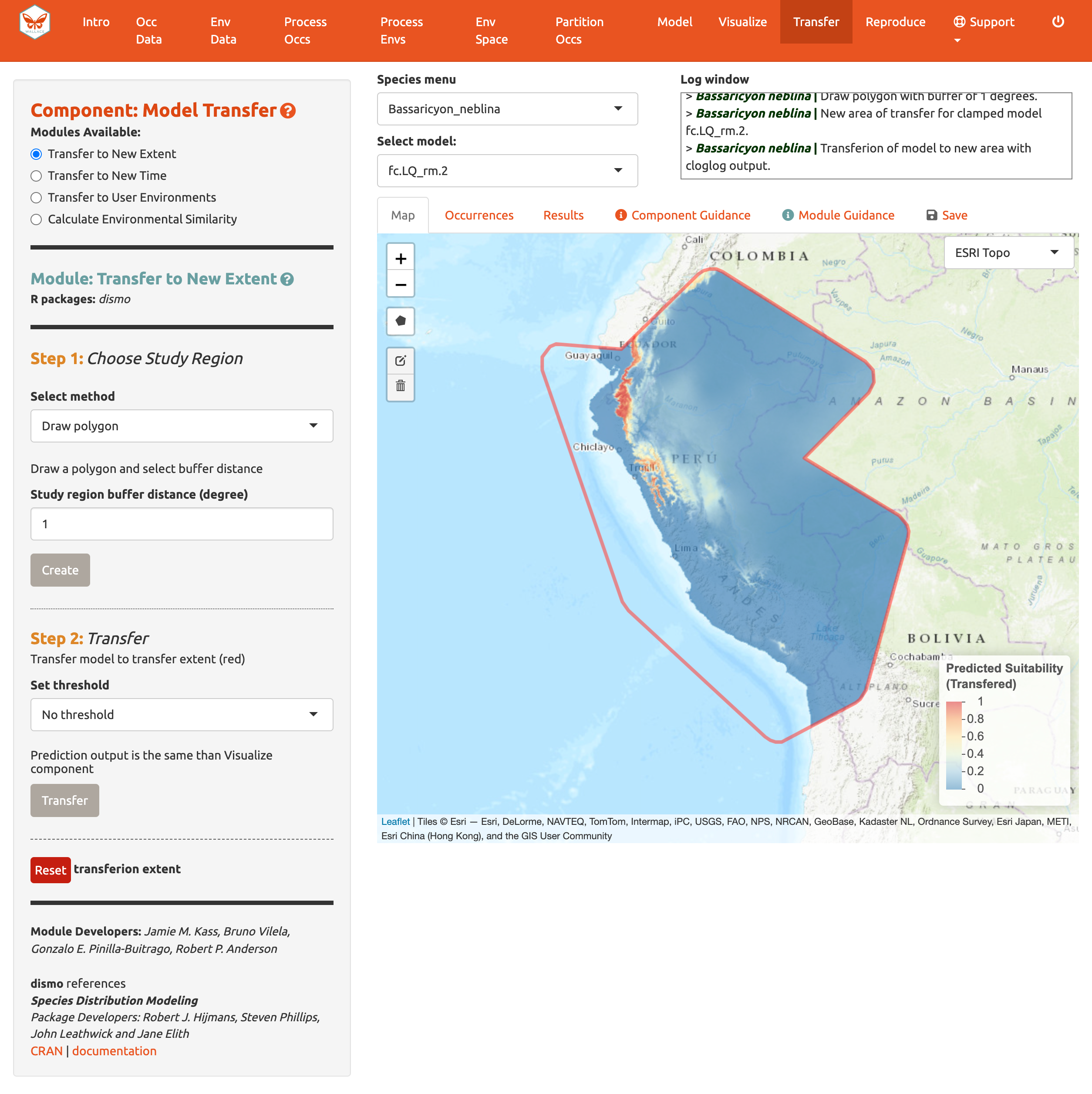
Let’s begin with Transfer to New Extent and see if Peru has suitable areas for the olinguito. In Step 1, use the polygon drawing tool to draw around Peru with a 1-degree buffer and hit “Create”. Alternatively, you can upload a shapefile or CSV file with records for vertices with fields “longitude, latitude” to use as a study region.

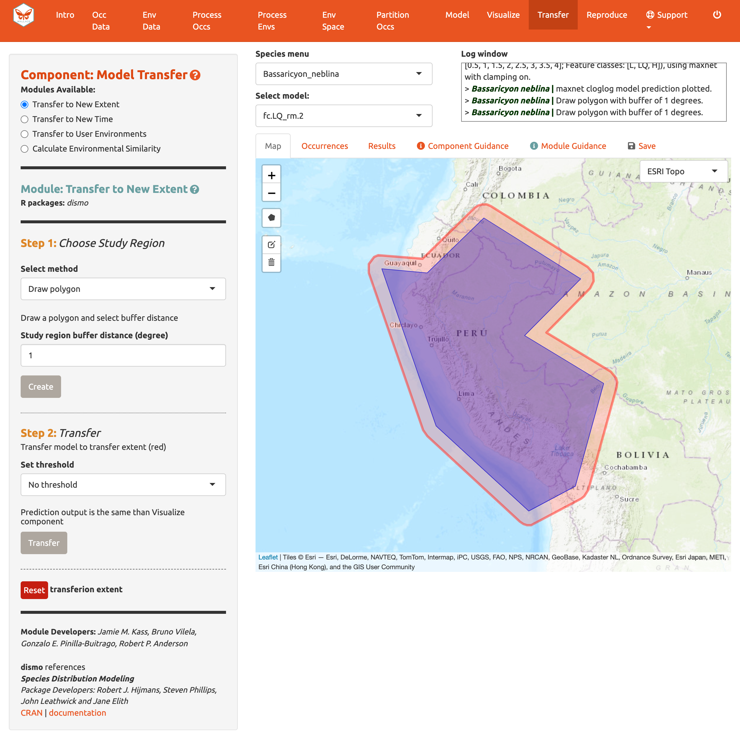
In Step 2, choose a threshold to make a binary prediction or no threshold for a continuous one and Transfer. Here, we see very low suitability for most of Peru for the olinguito.

Note: to remove the outline of the polygon from the prediction, click the Trashcan icon and “Clear all”.

If you initially used WorldClim or ecoClimate as environmental variables, you can use Transfer to New Time. In Step 1, there are three options to choose a study region; to draw a polygon, use the same extent, or upload a polygon. In Step 2, you have the choice of WorldClim or Ecoclimate for source variables. The choice depends on your initial selection of environmental variables in Component: Env Data. For WorldClim, select a time period, a global circulation model, a representative concentration pathway (RCP), and a threshold. Notice also that there are several global circulation models (GCMs) to choose from—these all represent different efforts to model future climate. Not all GCMs have raster data for each RCP. See the module guidance text for more on RCPs and GCMs. Note: some databases have phased out RCPs for Shared Socioeconomic Pathways (SSPs), so be advised that some literature might use SSP terminology instead of RCP. For ecoClimate, you can select a Atmospheric Oceanic General Circulation Model (AOGCM), temporal scenario, and threshold.

The third module, Transfer to User Environments, gives users the option to project their model to their own uploaded environmental data. The first step is the same as before (select the study region), but in the second step users can upload single-format rasters (.tif, .asc) to use as new data for model projection. The rasters must have the same extent and resolution (cell size), and the names of the files must correspond to the environmental variables used in modeling. To assist, there is a message “Your files must be named as: …” indicating the correct file names to use.

We will skip the Transfer to New Time and Transfer to User Environments and move on to to Calculate Environmental Similarity.
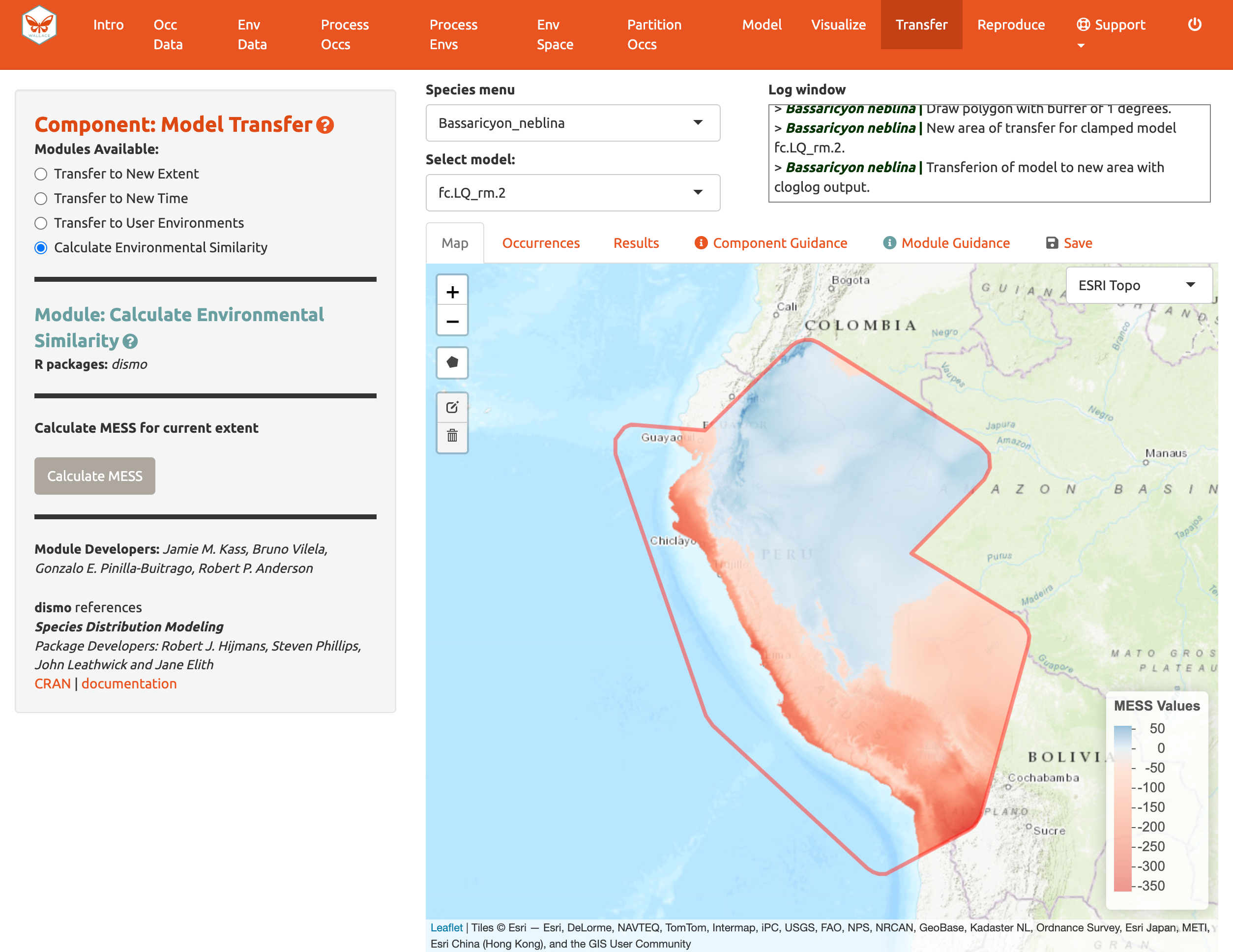
When transferring a model, there may be areas within our new ranges of values that have high uncertainty because they are very different from the values used in model-building. In order to visualize where these areas are, we can use the fourth module, Calculate Environmental Similarity, to plot a MESS map. MESS stands for (M)ultivariate (E)nvironmental (S)imilarity (S)urface, and the map shows a continuous scale of environmental difference from the training data used for model-building, where increasing positive values mean more similar (blue), and decreasing negative values mean more different (red); please see the module guidance text for details. We can see that future climate values at high elevation are more similar to our training data, whereas those at lower elevations towards the coast are very different in some places. We may therefore interpret that predicted suitability in these areas has higher uncertainty.

Reproduce

A major advantage of Wallace is reproducibility. The first option within this component is downloading code to run the analysis. While we were using Wallace, R code has been running in the background, evident from the messages printed to the R console. This option allows you to download a simplified version of this code in the form of a condensed and annotated R script. This script serves as documentation for the analysis and can be shared. It can also be run to reproduce the analysis, or edited to change aspects of it. The script can be downloaded as several file types, but the R Markdown format (.Rmd), which is a convenient format for combining R code and notation text, can be run directly in R. For .pdf downloads, the software TeX is necessary to be installed on your system. Please see the text on this page for more details.

To download the script, select Rmd and click Download.

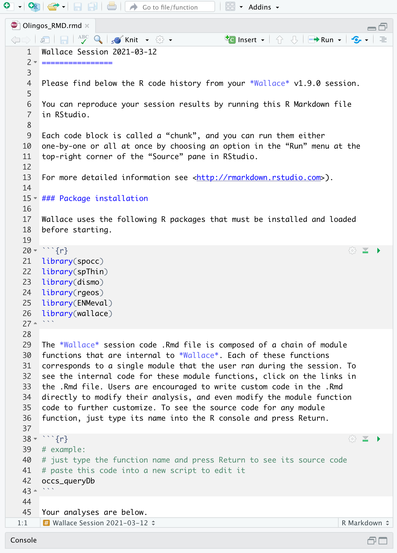
Now, you should have an .Rmd file that contains your complete analysis. Modules from Wallace are indicated as headers denoted by ###.

You might want to open a new R window and try running some of this code. Remember that later sections of code may depend on things that were done earlier, so they may not all run if you skip ahead. Note that any Env Space analysis will appear at the end of the file. Also remember that if you close your Wallace session you’ll lose your progress in the web browser (but your .Rmd will be unaffected). If you use RStudio, you can open this Rmd and click knit to compile your workflow into a shareable html document.

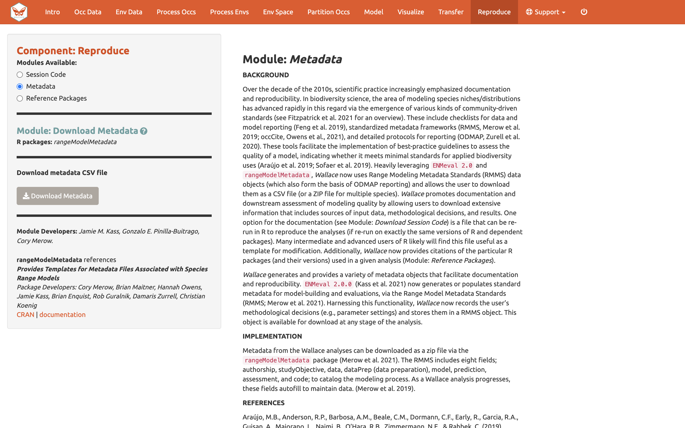
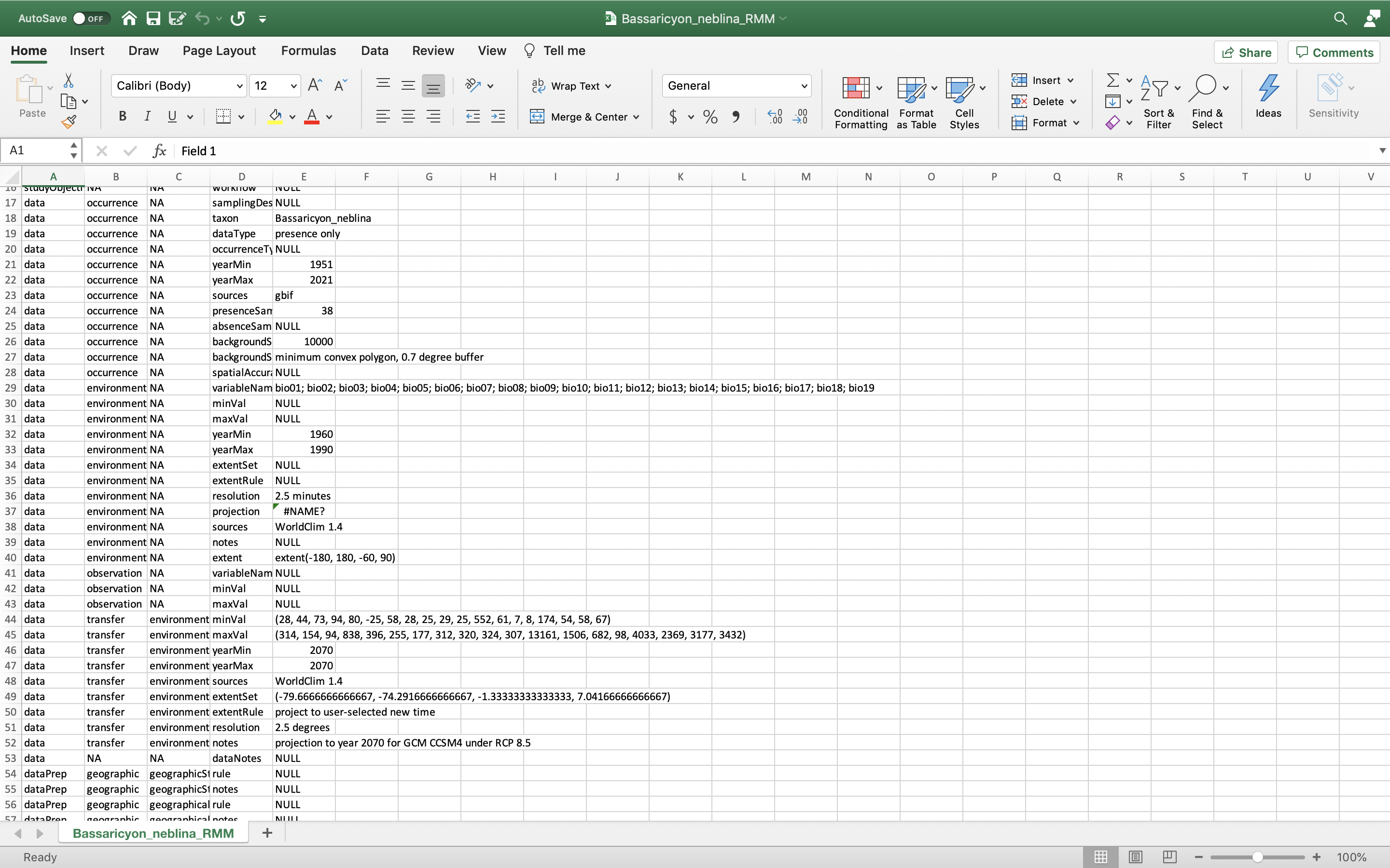
You can also download the Metadata. Wallace generates and provides a variety of metadata objects that facilitate documentation and reproducibility by recording the user’s methodological decisions (e.g., parameter settings) and stores them in a Range Model Metadata Standards object. This will download as a zip and contain a CSV file (.csv) for each species.

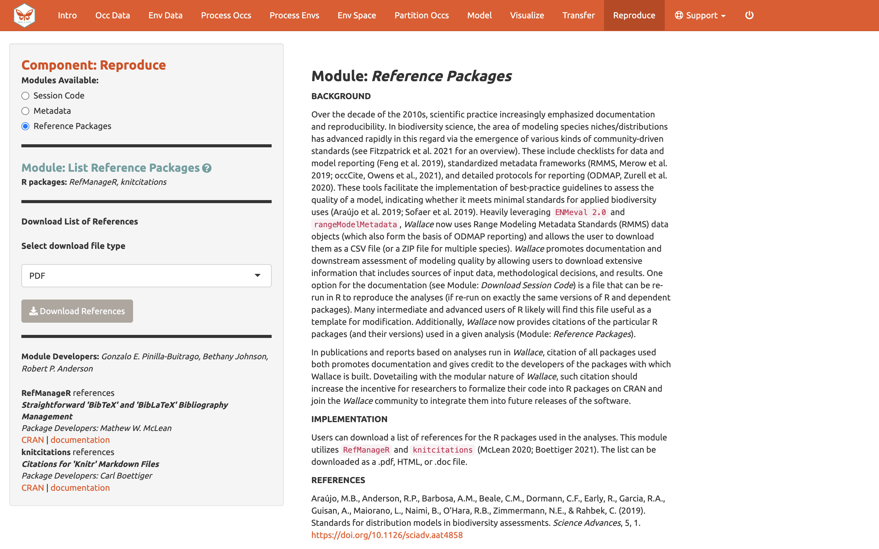
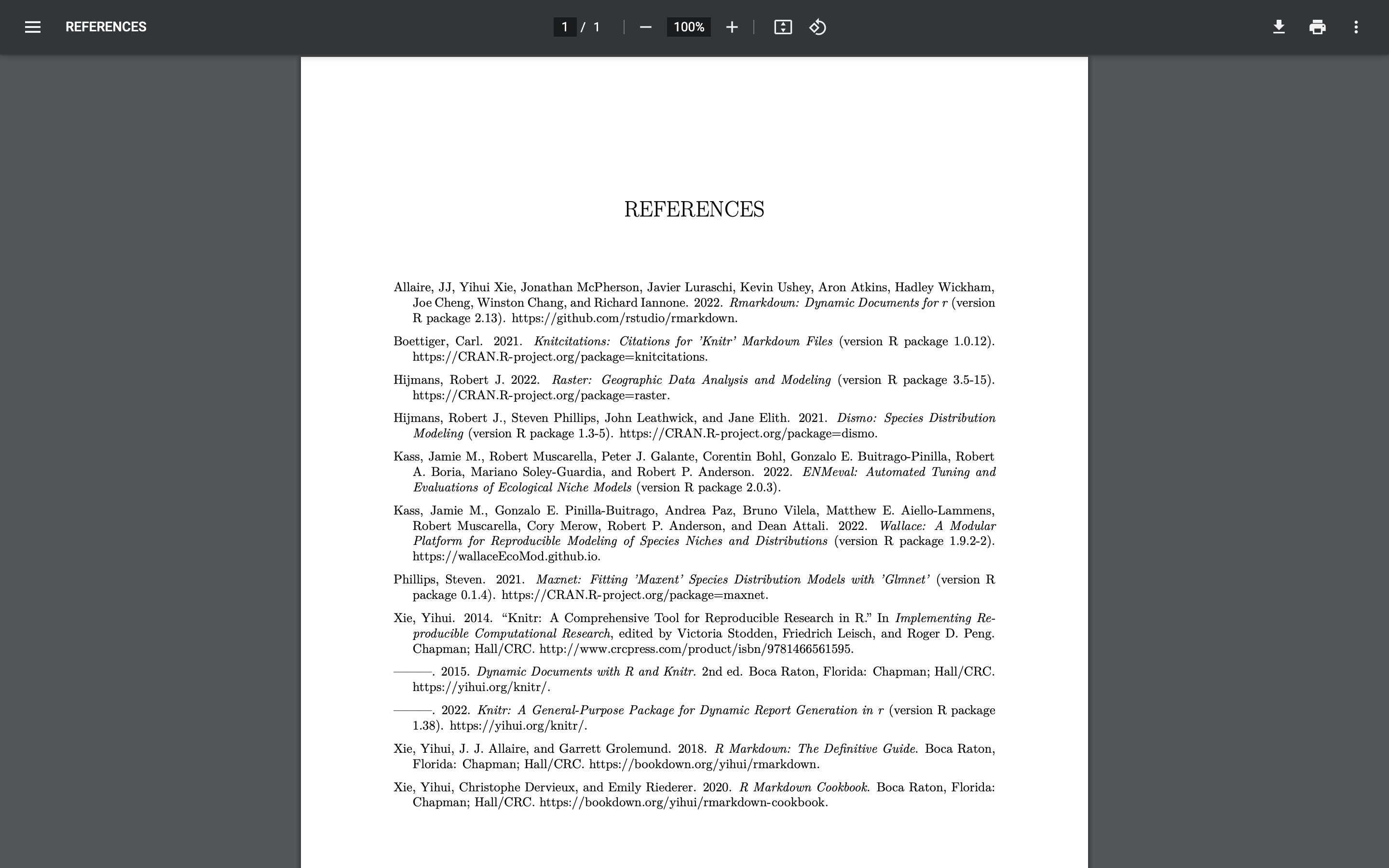
The last module available in the Reproduce component is Reference packages. Here, you can download the citations for all the R-packages used in the analysis. To give people credit for the underlying packages that make Wallace possible (and to document your analyses properly), it is critical to cite the packages and their version number. Remember, Wallace is modular and aims to facilitate access to and use of many R packages being produced by the biogeography research community. Please promote this by citing packages…and think about making one of your own and adding it to a future version of Wallace someday!

Conclusion

We are currently working with various partners on exciting additions, so stay tuned for future versions of Wallace. Until then, you can always work in R after the session by modifying the .Rmd and building on the analysis.

Thank you for following the Wallace v2 vignette. We hope you learned more about the updated application, its features, and modeling of species distributions and niches in general. We hate to be repetitive, but we highly encourage you to read the guidance text, follow up on the recommended publications, and hopefully let them lead you to other relevant publications that can inform you further. Also, remember to discuss these topics with your peers.

We encourage you to join the Wallace Google Group–we’d love to hear your thoughts, opinions, or suggestions on how to make Wallace better for all users. Members can post to the community and be updated on any future announcements. If you find a bug in the software, it can be reported on the GitHub issues page or using the bug reporting form.

Acknowledgments

Wallace was recognized as a finalist for the 2015 Ebbe Nielsen Challenge of the Global Biodiversity Information Facility (GBIF), and received prize funding.
This material is based upon work supported by the National Science Foundation under Grant Numbers DBI-1661510 (RPA; Robert P. Anderson), DBI-1650241 (RPA), DEB-1119915 (RPA), DEB-1046328 (MEA; Matthew E. Aiello-Lammens), DBI-1401312 (RM; Robert Muscarella), and funding from the National Aeronautics and Space Administration grant 80NSSC18K0406 (MEB; Mary E. Blair). Any opinions, findings, and conclusions or recommendations expressed in this material are those of the author(s) and do not necessarily reflect the views of the NSF or NASA.

Resources

Wallace website https://wallaceecomod.github.io/

ENM2020 W19T2 Online open access Ecological Niche Modeling Course by A.T. Peterson, summary of modeling, includes Walkthrough of Wallace V1 https://www.youtube.com/watch?v=kWNyNd2X1uo&t=1226s

Learn more about Olingos and the Olinguito https://www.ncbi.nlm.nih.gov/pmc/articles/PMC3760134/

Gerstner et al. (2018). Revised distributional estimates for the recently discovered olinguito (Bassaricyon neblina), with comments on natural and taxonomic history. https://doi.org/10.1093/jmammal/gyy012

References

Phillips, S.J., Anderson, R.P., Dudík, M., Schapire, R.E., Blair, M.E. (2017). Opening the black box: an open-source release of Maxent. Ecography, 40(7), 887-893. https://doi.org/10.1111/ecog.03049

Helgen et al Helgen, K., Kays, R., Pinto, C., Schipper, J. & González-Maya, J.F. (2020). Bassaricyon neblina (amended version of 2016 assessment). The IUCN Red List of Threatened Species 2020: e.T48637280A166523067. https://www.iucnredlist.org/species/48637280/166523067

Helgen, K., Kays, R., Pinto, C. & Schipper, J. (2016). Bassaricyon alleni. The IUCN Red List of Threatened Species 2016: e.T48637566A45215534. https://www.iucnredlist.org/species/48637566/45215534

Hijmans, R.J., Cameron, S.E., Parra, J.L., Jones, P.G., Jarvis, A. (2005). Very high resolution interpolated climate surfaces for global land areas. International Journal of Climatology, 25(15), 1965-1978. https://doi.org/10.1002/joc.1276

Lima-Ribeiro, M.S., Varela, S., González-Hernández, J., Oliveira, G., Diniz-Filho, J.A.F., Terribile, L.C. (2015). ecoClimate: a database of climate data from multiple models for past, present, and future for Macroecologists and Biogeographers. Biodiversity Informatics 10, 1-21. https://www.ecoclimate.org/

GBIF.org (2022). GBIF Home Page. Available from: https://www.gbif.org [19 April 2022].

Aiello-Lammens M.E., Boria R.A., Radosavljevic A., Vilela B., Anderson R.P. (2015). spThin: an R package for spatial thinning of species occurrence records for use in ecological niche models. Ecography, 38(5), 541-545. https://doi.org/10.1111/ecog.01132

Gerstner, B.E., Kass, J.M., Kays, R., Helgen, K.M., Anderson, R.P. (2018). Revised distributional estimates for the recently discovered olinguito (Bassaricyon neblina), with comments on natural and taxonomic history. Journal of Mammalogy, 99(2,3), 321-332. https://doi.org/10.1093/jmammal/gyy012

Kass, J., Muscarella, R., Galante, P.J., Bohl, C.L., Pinilla-Buitrago, G.E., Boria, R.A., Soley-Guardia, M., Anderson, R.P. (2021). ENMeval 2.0: Redesigned for customizable and reproducible modeling of species’ niches and distributions. Methods in Ecology and Evolution, 12(9), 1602-1608. https://doi.org/10.1111/2041-210X.13628

Merow, C., Smith, M.J., Silander, J.A. (2013). A practical guide to MaxEnt for modeling species’ distributions: What it does, and why inputs and settings matter. Ecography, 36(10), 1058-1069. https://doi.org/10.1111/j.1600-0587.2013.07872.x

Bethany A. Johnson, Gonzalo E. Pinilla-Buitrago, Andrea Paz, Jamie M. Kass, Sarah I. Meenan, Robert P. Anderson

2022-04-18; updated 2023-03-11